Polynomial magic I : Chebyshev polynomials

Orthogonal polynomials pop up everywhere in applied mathematics and in particular in numerical analysis. Within machine learning and optimization, typically (a) they provide natural basis functions which are easy to manipulate, or (b) they can be used to model various acceleration mechanisms.

In this post, I will describe one class of such polynomials, the Chebyshev polynomials (Tchebychev in French, Чебышёв in Russian), whose extremal properties (beyond being orthogonal) are useful in the analysis of accelerated algorithms.

Definition and first properties

The \(k\)-th Chebyshev polynomial \(T_k\) is classically defined as the unique polynomial such that $$\forall \theta \in [0,2\pi], \ \cos (k\theta) = T_k(\cos \theta).$$

Recurrence. Summing the two equations \(\cos [(k\pm 1)\theta] = \cos (k\theta) \cos \theta \mp \sin (k\theta) \sin \theta\), the following recurrence relationship can be deduced: $$\forall k >0, \ T_{k+1}(X) = 2X T_k(X) \, – T_{k-1}(X).$$

Together with the first two polynomials \(T_0 (X) = 1\) and \(T_1(X) = X\), this leads to \(T_2(X) = 2X^2 – 1\), \(T_3(X) = 4X^3 – 3X\), and so on.

From the recurrence relationships, one can easily deduce that \(T_k\) has the parity of \(k\) and that \(T_k\) has degree \(k\), with leading coefficient \(2^{k-1}\).

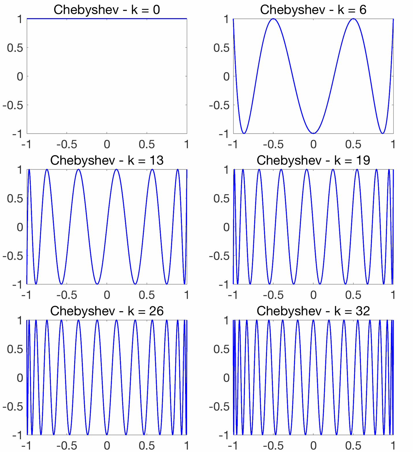
Oscillatory behavior. For \(k\theta = j \pi\), for \(j\) integer, we have \(\cos (k \theta)=(-1)^j\), while when \(j\) goes from \(k\) to \(0\), \(\cos \theta = \cos\! \big( \frac{ j \pi}{k}\big)\) goes from -1 to 1. Thus, on \([-1,1]\), \(T_k(x)\) oscillates between \(-1\) and \(1\), with equality for \(\cos\! \big( \frac{j \pi}{k} \big)\) for \(j = 0,\dots,k\). This oscillatory behavior is illustrated below and crucial for the extremal properties below.

Orthogonality. Using the orthogonality of the Fourier basis on \([0,2\pi]\), we have for \(k \neq \ell\), \(\int_0^{\pi} \cos (k\theta) \cos (\ell\theta) d\theta=0\), and with the change of variable \(x = \cos \theta\), we obtain $$\int_{-1}^1 \frac{T_k(x) T_\ell(x)}{\sqrt{1-x^2}} dx = 0.$$ Thus the Chebyshev polynomials inherit from many properties from such orthogonal polynomials (such as the two-term recursion above, but for the Chebyshev polynomials, these can obtained more directly). For further properties, see [1].

Extremal properties

Chebyshev polynomials exhibit many “extremal properties”, of the form: among all polynomials of degree \(k\) with some form of normalization (e.g., fixed \(k\)-th order coefficient or value at given point), the one with smallest specific norm is proportional to \(T_k\).

The most classical one is as follows: the polynomial \(P\) of degree \(k\) with \(k\)-th order coefficient equal to one, and with minimum \(\ell_\infty\)-norm \(\max_{ x \in [-1,1]} \! | P(x)|\) on \([-1,1]\), is \(P = \frac{1}{2^{k-1}}T_k\). The proof is particularly elegant and simple (see here). Since this is not the property that we need for optimization, we will consider another one.

Proposition (largest value outside of \([-1,1]\)). For any polynomial \(P\) of degree \(k\) such that \(|P(x)| \leq 1\) for \(x \in [-1,1]\), and any \(z > 1\), \(|P(z)| \leq T_k(z)\).

Proof. By contradiction, we assume that there exists \(z > 1\) such that \(P(z)>T_k(z)\) (the other possibility \(P(z) < -T_k(z)\) is done by replacing \(P\) by \(-P\)). Without loss of generality, we can assume that \(\max_{x \in [-1,1]} |P(x) | < 1\) (by potentially rescaling \(P\)). Then, the polynomial \(Q = P – T_k\) of degree \(k\) has alternatively strictly positive and negative values between \(-1\) and \(z>1\). Indeed, \(Q(z) > 0\), and \((-1)^j Q\big(\cos\! \big(\frac{j \pi}{k}\big)\big) < 0 \) for all \(j = 0,\dots,k\). Therefore there are \(k+2\) alternating signs, and thus \(k+1\) zeros, which implies that \(Q=0\) since \(Q\) has degree \(k\). This is a contradiction with the existence of \(z\).

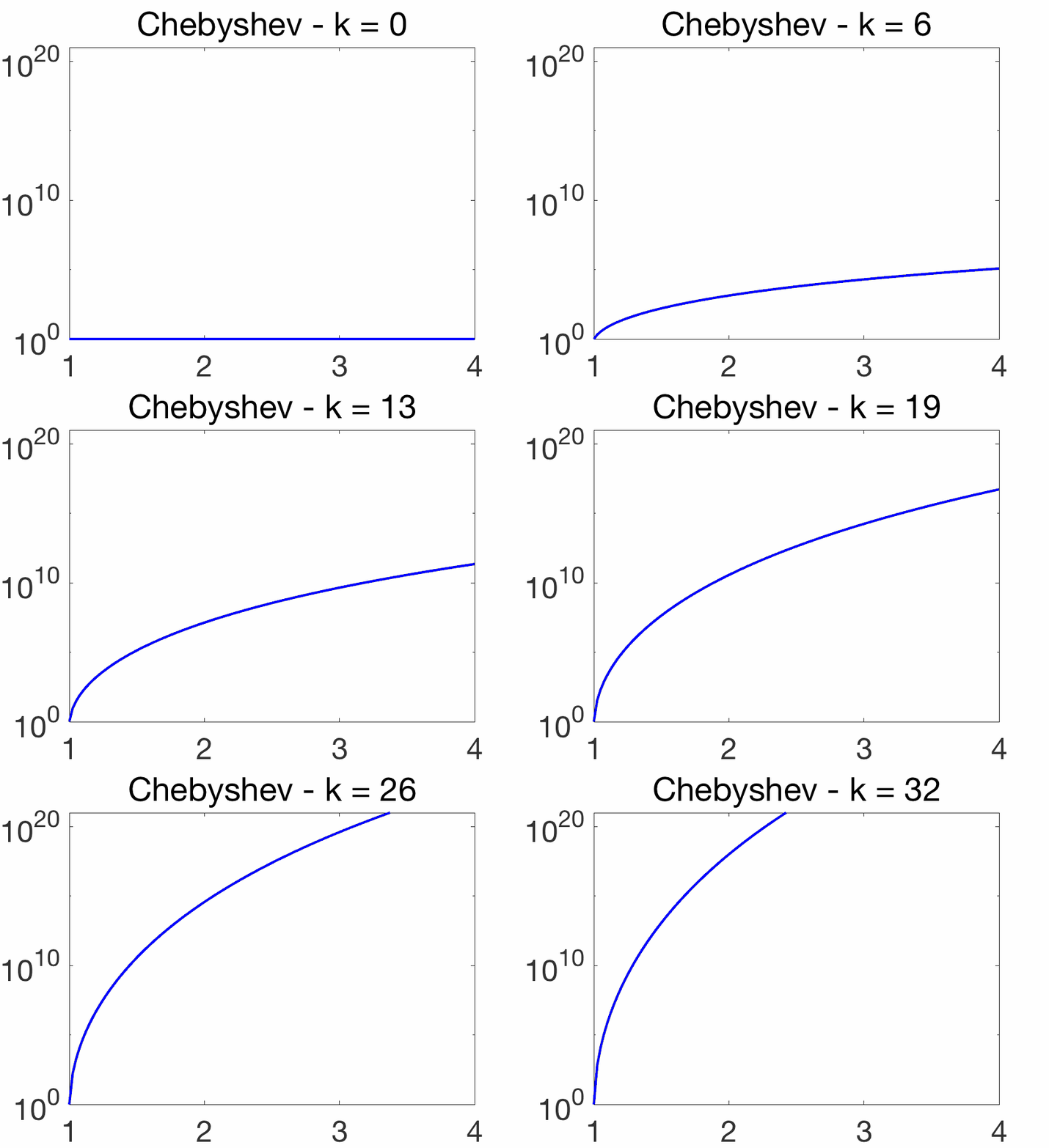
Note that for any \(\theta\), \(T_k( \cosh \theta) = \cosh (k\theta)\) (which can be shown by induction), and \(T_k\) is thus increasing on \([1,+\infty)\) with values quickly increasing as \(k\) grows. See an illustration below.

Chebyshev acceleration

We consider a recursion in \(\mathbb{R}^n\) of the form \(x_k = A x_{k-1} – b\), with \(A \in \mathbb{R}^{n \times n}\) a symmetric matrix and eigenvalues in \([-\rho,\rho]\) with \(\rho \in [0,1)\). Such recursions are ubiquitous in data science, as (1) gradient descent on a strongly-convex quadratic function, or (b) gossip for distributed averaging [2] (see an example in a section below).

The recursion converges to the unique (because \(\rho \in [0,1)\)) fixed point \(x_\ast \in \mathbb{R}^n\) such that \(x_\ast = A x_\ast – b\). We have, by unrolling the recursion: $$ x_k – x_\ast = A ( x_{k-1} – x_\ast) = A^k (x_0 – x_\ast).$$

This leads to the usual exponential convergence rate \(\| x_k – x_\ast\|_2 \leq \rho^k \| x_0 – x_\ast\|_2\). In the following, writing \(\rho = 1 – ( 1-\rho)\) makes explicit the importance of \(1-\rho\), which is the gap between \(1\) and the largest eigenvalue of \(A\). Increasing this gap is equivalent to accelerating the convergence rate.

In order to speed-up convergence, a classical idea is to take linear combinations of all past iterates. That is, we consider \(y_k = \sum_{i=0}^k \nu_i^k x_i\) for some weights \(\nu_i^k\) such that \(\sum_{i=0}^k \nu_i^k=1\) (so that if all iterates are already at \(x_\ast\), then the weighted average stays there). We have $$ y_k – x_\ast = \sum_{i=0}^k \nu_i^k ( x_i – x_\ast) = \sum_{i=0}^k \nu_i^k A^i (x_0-x_\ast) = P_k(A) (x_0-x_\ast),$$ where \(P_k(X) = \sum_{i=0}^k \nu_i^k X^i\) is a polynomial such that \(P_k(1)=1\). Therefore, we have: $$ \| y_k – x_\ast\|_2 \leq \max_{\lambda \in [-\rho, \rho]} |P_k(\lambda)| \cdot \|x_0 – x_\ast\|_2.$$

In order to select the best polynomial, we are looking for \(P_k\) such that \(P_k(1)=1\) and \(\max_{\lambda \in [-\rho,\rho]}\! |P_k(\lambda)|\) is as small as possible. Up to mapping \([-\rho,\rho]\) to \([-1,1]\), we know from the extremal property above that the optimal polynomial is exactly a rescaled Chebyshev polynomial, that is, $$P_k(X) = \frac{T_k(X/\rho)}{T_k(1/\rho)}.$$

The maximal value on \([-\rho,\rho]\) is then \((T_k(1/\rho))^{-1}\). In order to compare to \(\rho^k\) (no acceleration), we can provide an equivalent of \([T_k(1/\rho)]^{-1/k}\) as \(\frac{\rho}{ 1+ \sqrt{1-\rho^2}}\) (see end of the post). There is no real acceleration when \(\rho\) is bounded away from 1, but as \(\rho\) tends to \(1\), this can be shown (see also the end of the post) to be equivalent to \(1 – \sqrt{2(1\!-\!\rho)}\), with the usual “square root” acceleration: \(1\!-\!\rho\) is essentially replaced by \(\sqrt{1\!-\!\rho}\).

We thus get an acceleration, but as is, computing \(y_k\) seems to require to store all values of \(x_1,\dots,x_k\), which is not practical. Since there is a second-order recursion for Chebyshev polynomials, one can derive one as well, directly for the sequence \((y_k)\). A somewhat lengthy calculation (see end of the post) leads to the recursion $$ y_{k+1} = \omega_{k+1} ( Ay_{k} – b) + (1-\omega_{k+1}) y_{k-1}, $$
with a sequence \(\omega_{k+1}\) also defined by recursion as \(\omega_{k+1} = ( 1 – \frac{\rho^2}{4} \omega_k)^{-1}\), initialized with \(\omega_1 = 2\), \(y_0 = x_0\), \(y_1 = Ax_0 – b\). Therefore, on top of the usual computation of \(A y_k -b\), Chebyshev acceleration comes at no extra computational cost.

Simpler stationary recursion. In the recursion above, the parameter \(\omega_k\) varies with \(k\). A similar (then non totally optimal) acceleration can be obtained by replacing all \(\omega_k\)’s by their limit \(\omega\) when \(k\) tends to infinity, which is characterized by the equation \(\omega = ( 1-\frac{\rho^2}{4} \omega)^{-1}\) with smallest solutions \(\frac{ 1/\rho – \sqrt{1/\rho^2 -1}}{\rho/2}\) (see end of the post for detailed computations). The now stationary recursion then becomes $$ y_{k+1} = \omega ( Ay_{k} – b) + (1-\omega) y_{k-1}, $$ and is exponentially convergent with rate proportional to \(\rho \omega/2 = \frac{1}{1/\rho + \sqrt{ 1/\rho^2 – 1}} = \frac{\rho}{1+ \sqrt{ 1 – \rho^2}}\). Thus, the recursion is simpler and the final speed asymptotically the same as full Chebyshev acceleration.

Relationship with other acceleration mechanisms

Non-adaptive schemes. As seen above for an affine operator \(F:\mathbb{R}^n \to \mathbb{R}^n\) (i.e., \(F(x) = Ax-b\)), Chebyshev acceleration takes a recursion of the form $$x_{k+1} = F(x_{k}),$$ and linearly combines iterates; it ends up creating second-order recursions of the form $$ y_{k+1} = \omega_{k+1} F(y_k) + (1-\omega_{k+1}) y_{k-1}, $$ with the same fixed points. Other formats (with fixed point preservation) can be considered such as $$ y_{k+1} = F(y_k) + \delta_{k+1}(y_k – y_{k-1}),$$ or $$ y_{k+1} = F(y_k) + \delta_{k+1}(F(y_k) – F(y_{k-1})), $$ for some constants \(\delta_{k+1}\).

When \(F\) is affine, the format does not matter much (and all end up being essentially equivalent), but for gradient descent algorithms where \(F(x) = x – \gamma f'(x)\) for some non-quadratic function \(f\) and \(\gamma\) a step-size, there is a difference, the last one corresponding to Nesterov acceleration (see a nice post on it here), and the one before to classical momentum, also known as the heavy-ball method (see [3]).

Adaptive schemes. The methods above need to know the bound on the spectrum \(\rho\). They have to commit to such a value (which is typically only known through upper bounds) and cannot “get lucky”, that is, even if the best value \(\rho\) is known, they cannot benefit from additional better properties of the spectrum of \(A\) (e.g., clustered eigenvalues). The conjugate gradient method, which accesses the matrix \(A\) with the slightly stronger oracle of computing \(Ax\) any \(x\) (and not only \(Ax – b\)), or Anderson acceleration (which does not need a stronger oracle), are adaptive for similar problems [4, 5]. Again, Chebyshev polynomials are present; probably more on this in future posts!

Application to accelerated gossip

A interesting linear recursion pops out in distributed optimization, where we assume that computers or processors are placed in \(n\) nodes in a network, and the goal is to minimize an average of function \(f_1,\dots,f_n\), each of them only accessible by the corresponding node. The nodes are allowed to communicate messages along each edge of a network.

The simplest of such problem is the network averaging problem where \(f_i(\theta) = \frac{1}{2} (\theta – \xi_i)^2\), for a uni-dimensional parameter \(\theta\) and \(\xi \in \mathbb{R}^n\). The solution of this consensus is \(\theta_\ast = \frac{1}{n} \! \sum_{i=1}^n \! \xi_i\).

The gossip algorithm [2] consists in iteratively replacing the value \(\theta_i\) at a given node by a weighted average \(\sum_{j \sim i} W_{ij} \theta_j\) of the values at neighboring nodes (and node \(i\)). If all \(n\) nodes communicate simultaneously, then the vector \(\theta \) is replaced by \(W \theta\), hence a linear recursion $$ \theta_{k+1} = W \theta_{k},$$ initialized at \(\theta_0 = \xi\). Assuming that \(W\) is symmetric, with non-negative off-diagonal elements, and such that \(W 1_n = 1_n\) (where \(1_n \in \mathbb{R}^n\) is the vector of all ones), then all eigenvalues of \(W\) except the largest one are included in the interval \([-\rho, \rho]\), with \(\rho \in (0,1)\) for a connected graph. A simple such matrix \(W\) can be obtained from the adjacency matrix \(A\) of the graph, such that \(A_{ij} = 1\) if nodes \(i\) and \(j\) are connected, and zero otherwise, as \(W = I – \alpha L \), with \(L = {\rm Diag}(A 1_n) – A\) the Laplacian matrix and \(\alpha\) selected so that the eigenvalues are all between \(-\rho\) and \(\rho\), except one, which is equal to 1 (see values of \(\rho\) and \(\alpha\) at the end of the post). We will see below that this extra eigenvalue which is equal to one is in fact not a problem for analyzing the convergence of this network averaging procedure.

When applying the gossip matrix \(W\) iteratively to \(\theta_0 = \xi\), the projection on the eigensubspace corresponding to the unit eigenvalue is not changed, while all other projections on the other eigensubspaces converge to zero at rate at most \(\rho^k\). Thus \(\theta_k\) converges to the constant vector \(\frac{1}{n} 1_n 1_n^\top \xi\) at rate \(\rho^k\), and thus to a constant vector, with the average \(\frac{1}{n} \! \sum_{i=1}^n \! \xi_i\) in all components.

Given that we have a linear recursion, we can use Chebyshev acceleration defined above and obtain substantial improvements, as illustrated below. For the use of this acceleration within distributed optimization algorithms, see [6] and references therein.

Conclusion

Among classical classes of orthogonal polynomials, Chebyshev polynomials are special, because beyond being orthogonal, they satisfy extremal properties that are particularly useful in numerical analysis.

In future posts, I plan to go over Jacobi polynomials (which include Legendre, Gegenbauer and Chebyshev polynomials), Hermite polynomials, and finally Bernoulli polynomials (which are not orthogonal but still very special). For all of these, there are natural applications in machine learning.

Acknowledgements. I would like to thank Raphaël Berthier for proofreading this blog post and making good clarifying suggestions.

References

[1] John C. Mason, and David C. Handscomb. Chebyshev polynomials. Chapman and Hall/CRC, 2002.
[2] Stephen Boyd, Arpita Ghosh, Balaji Prabhakar, Devavrat Shah. Randomized gossip algorithms. IEEE/ACM Transactions on Networking, 14:2508-2530, 2006.
[3] Euhanna Ghadimi, Hamid Reza Feyzmahdavian, and Mikael Johansson. Global convergence of the heavy-ball method for convex optimization. European Control Conference (ECC), 2015.
[4] Homer F. Walker, Peng Ni. Anderson acceleration for fixed-point iterations. SIAM Journal on Numerical Analysis, 49(4):1715-1735, 2011.
[5] Damien Scieur, Alexandre d’Aspremont, Francis Bach. Regularized Nonlinear Acceleration. Mathematical Programming, 2018.
[6] Kevin Scaman, Francis Bach, Sébastien Bubeck, Yin-Tat Lee, Laurent Massoulié. Optimal algorithms for smooth and strongly convex distributed optimization in networks. Proceedings of the International Conference on Machine Learning (ICML), 2017.
[7] Mieczysław A. Kłopotek. Spectral Analysis of Laplacians of an Unweighted and Weighted Multidimensional Grid Graph — Combinatorial versus Normalized and Random Walk Laplacians. Technical report, ArXiv:1707.05210, 2019.

Detailed Computations

Limit of \([T_k(1/\rho)]^{-1/k}\). For \(z \geq 1\), then a well-known property of Chebyshev polynomials is that \(T_k(z) = \cosh [ k \, {\rm acosh} (z)]\) (which can be shown by induction using basic hyperbolic trigonometry identities). Moreover, we have \({\rm acosh} (z) = \log( z + \sqrt{z^2-1} )\) and thus $$T_k(z) = \frac{1}{2} \big[ \big( z + \sqrt{z^2-1} \big)^k + \big(z – \sqrt{z^2-1}\big)^k \big].$$ For \(z = 1/\rho\), and taking limits, we get that \([T_k(z)]^{1/k}\) tends to \( z + \sqrt{z^2-1}\), which leads to the limit \(\frac{\rho}{ 1+ \sqrt{1-\rho^2}}\) for \([T_k(z)]^{-1/k}\). Then a classical Taylor expansion in \(1-\rho\) leads to \(1 – \sqrt{2(1-\rho)}\).

Recurrence for Chebyshev acceleration. We have, using the recursion for Chebyshev polynomials $$y_{k+1} – x_\ast = \frac{ 2 }{T_{k+1}(1/\rho)} (A/\rho) T_k(A/\rho) ( x_0 – x_\ast) \ – \frac{ 1 }{T_{k+1}(1/\rho)} T_{k-1}(A/\rho) ( x_0 – x_\ast).$$ Using the equality \(x_\ast = A x_\ast -b\), the terms in \(x_\ast\) cancel (they have to anyway, because \(P_k(1)=1\)). We then get $$y_{k+1} = \frac{ (2/\rho) T_{k}(1/\rho)}{T_{k+1}(1/\rho)} ( A y_k – b) \, – \frac{ T_{k-1}(1/\rho) }{T_{k+1}(1/\rho)} y_{k-1}.$$

Using \(T_{k-1}(1/\rho) = (2/\rho) T_{k}(1/\rho) – T_{k+1}(1/\rho)\), and denoting \(\omega_{k+1} = \frac{ (2/\rho) T_{k}(1/\rho)}{T_{k+1}(1/\rho)}\), we get $$y_{k+1} = \omega_{k+1} ( A y_{k} – b) + ( 1- \omega_{k+1}) y_{k-1}.$$ Reusing one last time the Chebyshev recursion, we get $$\omega_{k+1}^{-1} = \frac{T_{k+1}(1/\rho)}{ (2/\rho) T_{k}(1/\rho)}= 1 – \frac{T_{k-1}(1/\rho)}{ (2/\rho) T_{k}(1/\rho)} =1 – \frac{\rho^2}{4} \omega_{k},$$ which is the desired recursion.

Convergence of stationary recursion. The roots of \(\omega = ( 1-\frac{\rho^2}{4} \omega)^{-1}\) are the ones of \(\frac{\rho^2}{4} \omega^2 – \omega + 1 = 0\), with smallest solutions \(\omega = \frac{ 1/\rho – \sqrt{1/\rho^2 -1}}{\rho/2}\). In order to study the second-order recursion $$ y_{k+1} = \omega ( Ay_{k} – b) + (1-\omega) y_{k-1}, $$ with constant coefficient, we need to compute the roots of \(r^2 = \omega \lambda r + (1-\omega)\), for \(|\lambda| \leq \rho\). The discriminant of this equation is \(\lambda^2 \omega^2 + 4 (1-\omega) \leq \rho^2 \omega^2 + 4(1-\omega) = 0\), and thus the roots are complex conjugate with squared modulus \((\omega\ – 1) = \frac{1}{4} \rho^2 \omega^2\) independent of \(\lambda\). Thus, as \(k\) tends to infinity, \(\| y_k – x_\ast\|_2^{1/k}\) tends to \(\frac{1}{2} \rho \omega = ( 1/\rho – \sqrt{ 1/\rho^2 – 1} ) = \frac{1}{1/\rho + \sqrt{ 1/\rho^2 – 1}}\), which is exactly the rate for Chebyshev acceleration.

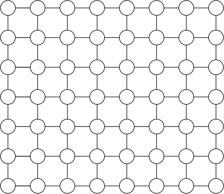
Eigenvalues of the Laplacian matrix of a square grid. Given a chain of length \(m\) such as depicted below, the \(m \times m\) Laplacian matrix can be shown (see [7]) to have eigenvalues \(2 + 2 \cos \frac{k\pi}{m}\) for \(k =1,\dots,m\).

For a two-dimensional grid of size \(m \times m\), then the \(m^2 \times m^2\) Laplacian matrix can be shown (see [7]) to have eigenvalues \(4 + 2\cos \frac{k_1\pi}{m} + 2\cos \frac{k_2\pi}{m}\) for \(k_1,k_2 =1,\dots,m\). Therefore, the second smallest eigenvalue is \(\lambda_\min = 2 – 2 \cos \frac{\pi}{m}\) and the largest eigenvalue is \(\lambda_\max = 4 + 4 \cos \frac{\pi}{m}\). We then select \(\alpha\) such that \(1-\alpha \lambda_\min = \rho\) and \(1-\alpha \lambda_\max = -\rho\), leading to \(\alpha = \frac{2}{\lambda_\min + \lambda_\max} = \frac{2}{6 + 2 \cos \frac{\pi}{m}}\) and finally \(\rho = \frac{\lambda_\max – \lambda_\min}{\lambda_\max + \lambda_\min} = \frac{2 +6 \cos \frac{\pi}{m} }{6 + 2 \cos \frac{\pi}{m}}\sim \frac{8 – 3 \frac{\pi^2}{m^2}}{8 – \frac{\pi^2}{m^2}}\sim 1 – \frac{\pi^2}{4 m^2}\). Thus, as a function of \(n = m^2\), the eigengap is proportional to \(1/n\).

More generally, for the grid of size \(m\) in dimension \(d\), then we get \(\lambda_\min = 2 – 2 \cos \frac{\pi}{m}\) and \(\lambda_\max = 2d + 2d \cos \frac{\pi}{m}\), and \(\rho = \frac{\lambda_\max – \lambda_\min}{\lambda_\max + \lambda_\min} = \frac{2d-2 +(2d+2) \cos \frac{\pi}{m} }{2d+2 + (2d-2) \cos \frac{\pi}{m}}\sim \frac{4d – (d+1) \frac{\pi^2}{m^2}}{4d – (d-1)\frac{\pi^2}{m^2}}\sim 1 – \frac{\pi^2}{2d m^2}.\) Thus, as a function of \(n = m^d\), the eigengap is proportional to \(1/n^{2/d}\). Moreover, when \(m\) is large, the normalizing factor \(\alpha\) tends to \(1/(2d)\).