The sum of a geometric series is all you need!

I sometimes joke with my students about one of the main tools I have been using in the last ten years: the explicit sum of a geometric series. Why is this?

From numbers to operators

The simplest version of this basic result for real numbers is the following: $$ \forall r \neq 1, \ \forall n \geq 0, \ \sum_{k=0}^n r^k = \frac{1-r^{n+1}}{1-r},$$ and is typically proved by multiplying the two sides by \(1-r\) and forming a telescoping sum. When \(|r|<1\), we can let \(n\) tend to infinity and get $$ \forall |r| < 1, \ \sum_{k=0}^\infty r^k = \frac{1}{1-r}.$$

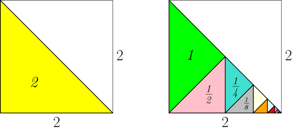
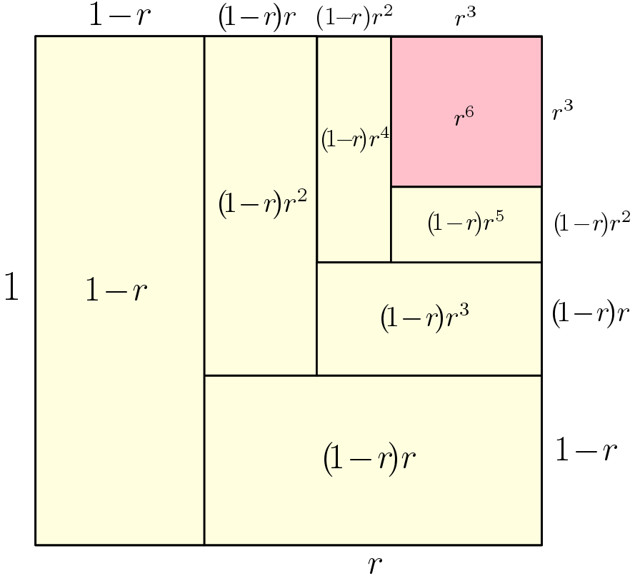
Proofs without words. There is a number of classical proofs of the last identities, many of them without words, presented in the beautiful series of books by Roger Nelsen [1, 2, 3]. I particularly like the two below.

High school: from philosophy to trigonometry. Before looking at extensions beyond real numbers, I can’t resist mentioning some of Zeno’s paradoxes, like Achilles and the tortoise, which are intimately linked with the sum of a geometric series (and which were a highlight of my high school philosophy “career”).

Speaking of high school, it is interesting to note that there, the core identity of this blog post, is often used as \(a^{n+1}-b^{n+1} = (a-b)(a^n+a^{n-1}b+\cdots+ab^{n-1}+b^{n})\) in order to factorize polynomials (and not in the other way around like done later in this post).

Another nice elementary use of geometric series comes up with complex numbers, in order to compute sum of cosines, such as: $$\! \sum_{k=0}^n \! \cos k\theta = {\rm Re} \Big(\!\sum_{k=0}^n e^{ i k \theta}\!\Big) = {\rm Re} \Big(\!\frac{e^{i(n+1)\theta}-1}{e^{i\theta}-1}\!\Big) = {\rm Re} \Big(\! \frac{ \sin \frac{n+1}{2} \theta e^{i(n+1)\theta/2}}{ \sin \frac{\theta}{2} e^{i\theta/2} }\!\Big) = \frac{ \sin \frac{n+1}{2} \theta}{\sin \frac{\theta}{2}} \cos \frac{n\theta}{2}. $$

Square matrices and operators. Within applied mathematics, the matrix and operator versions are the most useful. For \(A\) a square matrix or any linear operator, we have $$ \forall A \mbox{ such that } I-A \mbox{ is invertible}, \ \sum_{k=0}^n A^k = (I-A)^{-1}(I-A^{n+1}),$$ with the classical proof: \(\displaystyle (I – A)\sum_{k=0}^n A^k = \sum_{k=0}^n A^k – \sum_{k=1}^{n+1} A^k = I – A^{n+1}.\)

When \(\| A\| <1\) for any matrix norm induced from a vector norm, we can let \(n\) go to infinity, to obtain the Neumann series \(\displaystyle \sum_{k=0}^{+\infty} A^k = (I-A)^{-1}\).

We are now ready to talk about machine learning and optimization!

Stochastic gradient for quadratic functions

Matrix geometric series come up naturally when analyzing iterative algorithms based on linear recursions. In this blog post, I will focus on stochastic gradient descent (SGD) techniques to solve the following problem: $$ \min_{\theta \in \mathbb{R}^d} F(\theta) = \frac{1}{2} \mathbb{E} \big[ y – \theta^\top \Phi(x) \big]^2,$$ where the expectation is taken with respect to some joint distribution on \((x,y)\). We denote by \(\theta_\ast \in \mathbb{R}^d\) the minimizer of the objective function above (which is assumed to exist). We assume the feature vector \(\Phi(x)\) is high-dimensional, so that the moment matrix \(H = \mathbb{E} \big[ \Phi(x)\Phi(x)^\top \big]\) cannot be assumed to be invertible.

Stochastic gradient descent recursion. Starting from some initial guess \(\theta_0 \in \mathbb{R}^d\), typically \(\theta_0 =0\), the SGD recursion is: $$ \theta_n = \theta_{n-1} – \gamma ( \theta_{n-1}^\top \Phi(x_n) \, – y_n) \Phi(x_n),$$ where \((x_n,y_n)\) is an independent sample from the distribution mentioned above, and \(\gamma > 0\) is the step-size. This algorithm dates back to Robbins and Monro in the 50’s and is particularly adapted to machine learning as it updates the parameter \(\theta\) after each observation \((x_n,y_n)\) (as opposed to waiting for a full pass over the data).

Denoting \(\varepsilon_n = y_n – \theta_\ast^\top \Phi(x_n)\) the residual between the observation \(y_n\) and the optimal linear prediction \(\theta_\ast^\top \Phi(x_n)\), we can rewrite the SGD recursion as $$\theta_n = \theta_{n-1} – \gamma ( \theta_{n-1}^\top \Phi(x_n) \, – \theta_{\ast}^\top \Phi(x_n) -\, \varepsilon_n) \Phi(x_n),$$ leading to $$\theta_n \, – \theta_\ast = \big[ I – \gamma \Phi(x_n) \Phi(x_n)^\top \big] ( \theta_{n-1}- \theta_\ast) + \gamma \varepsilon_n \Phi(x_n).$$

This is a stochastic linear recursion on the deviation to optimum \(\theta_n \, – \theta_\ast\). The expectation of the SGD recursion is: $$\mathbb{E} [ \theta_n] \, – \theta_\ast = \big[ I – \gamma H \big] ( \mathbb{E}[ \theta_{n-1}] – \theta_\ast), $$ where \(H = \mathbb{E} \big[ \Phi(x) \Phi(x)^\top \big]\), and where we have used that \(\gamma \varepsilon_n \Phi(x_n)\) has zero expectation (as a consequence of optimality conditions for \(\theta_\ast\)). This is exactly the gradient descent recursion on the expected loss (which cannot be run in practice because we only have access to a finite amount of data).

Simplification. The main difficulty in analyzing the stochastic recursion is the presence of two sources of randomness when compared to the gradient descent recursion: (A) some additive noise \(\gamma \varepsilon_n \Phi(x_n)\) independent of the current iterate \(\theta_{n-1}\) and with zero expectation, and (B) some multiplicative noise \(\gamma \big[ H – \Phi(x_n) \Phi(x_n)^\top \big] (\theta_{n-1} – \theta_\ast)\), which comes from the use of \( I – \gamma \Phi(x_n) \Phi(x_n)^\top \) instead of \(I – \gamma H\), and depends on the current iterate \(\theta_{n-1}\).

In this blog post, for simplicity, I will ignore the multiplicative noise and only focus on the additive noise, and thus consider the recursion $$\theta_n\, – \theta_\ast = ( I – \gamma H ) ( \theta_{n-1}- \theta_\ast) + \gamma \varepsilon_n \Phi(x_n).$$ Detailed studies with multiplicative noise can be found in [4, 5, 6, 7], and lead to similar results. Moreover, I will assume (again for simplicity) that \(\varepsilon_n\) and \(\Phi(x_n)\) are independent, and that \(\mathbb{E} [ \varepsilon_n^2 ] = \sigma^2\) (which corresponds to uniform noise of variance \(\sigma^2\) on top of the optimal linear predictions); again, results directly extends without this assumption.

Bias / variance decomposition. Having a constant multiplicative term \(I – \gamma H\) in the recursion leads to an explicit formula: $$\theta_n – \theta_\ast = ( I – \gamma H ) ^n ( \theta_{0}- \theta_\ast) + \sum_{k=1}^n \gamma ( I – \gamma H ) ^{n-k} \varepsilon_k \Phi(x_k),$$ which is now easy to analyze. It is the sum of a deterministic term depending on initial conditions, and a zero mean term which is the sum of independent zero-mean terms due to the noise in the gradients. Thus, we can compute the expectation of the excess risk \(F(\theta_n)\, – F(\theta_\ast) = \frac{1}{2} ( \theta_n – \theta_\ast)^\top H ( \theta_n – \theta_\ast)\), as follows: $$\! \mathbb{E} \big[ F(\theta_n) \,- F(\theta_\ast)\big] = {\rm Bias} + { \rm Variance}, $$ where the bias term characterizes the forgetting of initial conditions: $$ {\rm Bias} = \frac{1}{2} ( \theta_0 – \theta_\ast)^\top ( I – \gamma H ) ^{2n} H ( \theta_0 – \theta_\ast), $$ and the variance term characterizes the effect of the noise: $${\rm Variance} = \frac{\gamma^2 }{2}\! \sum_{k=1}^n \! \mathbb{E} \big[ \varepsilon_k^2 \Phi(x_k)^\top ( I – \gamma H ) ^{2n-2k}H \Phi(x_k) \big] = \frac{\gamma^2 \sigma^2}{2}\! \sum_{k=1}^n \! {\rm tr} \big[ ( I – \gamma H ) ^{2n-2k}H^2 \big] .$$

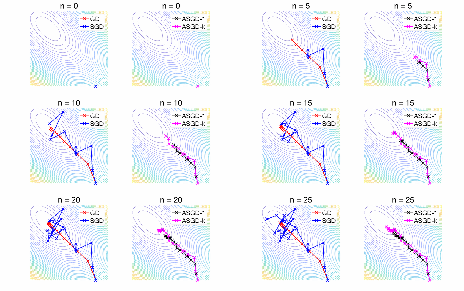
The bias term is exactly the convergence rate of gradient descent on the expected risk, and can be controlled by upper-bounding the eigenvalues of the matrix \(( I – \gamma H ) ^{2n} H\). As shown at the end of the post, when \(\gamma \leq \frac{1}{L}\), where \(L\) is the largest eigenvalue of \(H\), then this matrix has all eigenvalues less than \(1/(4n\gamma)\), leading to a bound on the bias term of $$ \frac{1}{8 \gamma n} \|\theta_0 – \theta_\ast\|^2.$$ We recover the traditional \(O(1/n)\) convergence rate of gradient descent. For the variance term we use the sum of a geometric series, to obtain the bound $$\frac{\gamma^2 \sigma^2}{2} {\rm tr} \big[ H^2( I – (I – \gamma H)^2 )^{-1} \big] = \frac{\gamma^2 \sigma^2}{2} {\rm tr} \big[ H^2( 2\gamma H – \gamma^2 H^2 )^{-1} \big] \leq \frac{\gamma \sigma^2}{2} {\rm tr}(H) .$$ While the bias term that characterizes the forgetting of initial conditions goes to zero as \(n\) goes to infinity, this is not the case for the variance term. This is the traditional lack of convergence of SGD with a constant step-size. In the left plot of the figure below, we compare deterministic gradient descent to stochastic gradient with a constant step-size. For convergence rates in higher dimension, see further below.

Convergence can be obtained by using a decreasing step-size, typically of the order \(1 / \sqrt{n},\) leading to an overall convergence rate proportional to \(1 / \sqrt{n}.\) This can be improved through averaging, which I now present.

Impact of averaging

We consider the averaged iterate \(\bar{\theta}_n = \frac{1}{n+1} \sum_{k=0}^n \theta_k\), an off-line (no interaction with the stochastic recursion) averaging often referred to as Polyak–Ruppert averaging, after [8, 9]. The averaged iterate can also be expressed as a linear function of initial conditions and noise variables as $$\bar{\theta}_n -\theta_\ast = \frac{1}{n+1} \sum_{k=0}^n ( I – \gamma H ) ^k ( \theta_{0}- \theta_\ast) + \frac{\gamma}{n+1} \sum_{k=1}^n \sum_{j=k}^n ( I – \gamma H ) ^{j-k} \varepsilon_k \Phi(x_k).$$ Geometric series come in again! We can get a closed form for \(\bar{\theta}_n -\theta_\ast\) as: $$\frac{1}{n+1} (\gamma H)^{-1} \big[ I – ( I – \gamma H ) ^{n+1} \big] ( \theta_{0}- \theta_\ast) + \frac{\gamma}{n+1} (\gamma H)^{-1} \sum_{k=1}^n \big[ I – ( I – \gamma H ) ^{n-k+1} \big] \varepsilon_k \Phi(x_k).$$

The bound on \(\mathbb{E} \big[ F(\bar{\theta}_n) \,- F(\theta_\ast)\big] \), will here also be composed of a bias term and a variance term.

Bias. The bias term is equal to $$\frac{1}{2(n+1)^2}( \theta_{0}- \theta_\ast) ^\top (\gamma H)^{-2} H \big[ I – ( I – \gamma H ) ^{n+1} \big]^2 ( \theta_{0}- \theta_\ast).$$ Using the fact that the eigenvalues of the matrix \( (\gamma H)^{-2} H \big[ I – ( I – \gamma H ) ^{n+1} \big]^2\) are all less than \((n+1)/\gamma\) (see proof at the end of the post), we obtain the upper bound $$ \frac{1}{2 (n+1)\gamma} \| \theta_0 – \theta_\ast\|^2,$$ which is essentially the same than with averaging (but, see an important difference in the discussion below, regarding the behavior for large \(n\)).

Variance. The variance term is equal to $$ \frac{\gamma^2}{2 (n+1)^2} \sum_{k=1}^n \sigma^2 {\rm tr} \Big( \big[ I – ( I – \gamma H ) ^{n-k+1} \big]^2 (\gamma H)^{-2} H^2 \Big).$$ Using the positivity of the matrix \(( I – \gamma H )\), we finally obtain the following bound for variance term: $$ \frac{ \sigma^2 n {\rm tr}(I)}{2(n+1)^2}\leq \frac{\sigma^2 d}{2n}.$$ We now have a convergent algorithm, and we recover traditional quantities from the statistical analysis of least-squares regression.

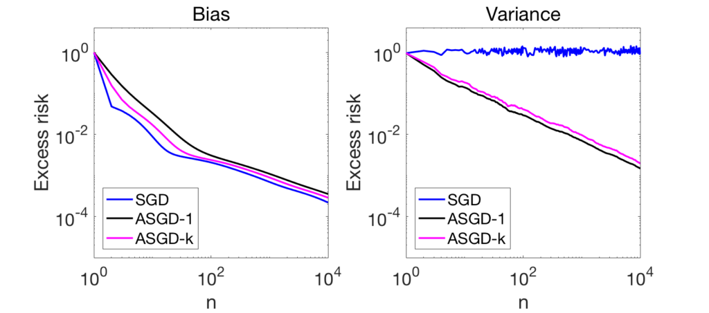
Experiments. Now, both bias and variance are converging at rate \(1/n\). See an illustration in two dimensions in the right plot of the figure above, as well as a convergence rates below. In these two figures, what differs is the decay of eigenvalues of \(H\) (fast in the first figure, slower in the second).

We can make the following observations:

• Depending on the amount of noise in the gradients, the sum of the variance and the bias terms will either be dominated by one of the two; typically the bias term in early iterations, and then the variance term (see more details in [5]).
• The variance term of non-averaged SGD is converging to a constant (while the bias term is exactly the one of regular gradient descent).
• With averaging, the variance terms decay as a line in a log-log plot. The reader with good eyes can check that the slope is indeed -1, thus illustrating the convergence rate in \(1/n\) (here the bound is tight). For the variance terms (right plots), there is no significant difference between the two eigenvalue decays.
• The bias terms have different behaviors for the two decays. For the fast decays (top plot), the bounds in \(1/n\) are reasonably tight (lines of slope -1). For slower decay, we see some strong-convexity behavior entering the scene, as the slowest eigenvalue is 1/100 and the number of iterations is far larger than 100, and thus the optimization problem looks strongly convex, and then the bias term of plain SGD (which corresponds to deterministic gradient descent) converges exponentially fast, while the two averaging techniques decay as powers of \(n\) (again, the acute reader can spot slopes of -2 and -4, and the smart reader can explain why; more on this in a future post dedicated to SGD).

Pros and cons of averaging. Overall, we can see that averaging may slow down the forgetting of initial conditions, while it makes the method robust to noise in the gradients. The trade-off depends on the amount of noise, but in most high-dimensional learning problems and for the accuracies practitioners are interested in (no need to have an excess risk of \(10^{-5}\) then the best risk is of order \(10^{-1}\)), the bias term is the one which is seen the most. Thus, a less-aggressive form of averaging that puts more weights on later iterates seems advantageous (pink curve above). More on this in a future blog post.

Beyond least-squares. In this blog post, to illustrate the use of sums of geometric series, I have focused on an idealized version (no multiplicative noise) of least-squares regression. For other losses, e.g., logistic loss, the analysis is more involved, and averaging does not lead to a converging algorithm, but transforms a term in \(\gamma\) into a term in \(\gamma^2\), which is still a significant improvement when the step-size \(\gamma\) is small (see [10] for more details).

Extensions

The sum of a geometric series can be extended in a variety of ways. For example, we can take the derivative with respect to \(r\), to get $$ \forall r \neq 1, \ \sum_{k=1}^n k r^{k-1} = \frac{1-r^{n+1}}{(1-r)^2} – \frac{ (n+1) r^n}{1-r} = \frac{1 + n r^{n+1} – (n+1) r^n }{(1-r)^2}.$$ This is useful for example to compute the performance of the weighted average \(\frac{2}{n(n+1)} \sum_{k=1}^n k \theta_k\). This can be extended further with the binomial series $$ (1-r)^{-1-\beta} = \sum_{k=0}^\infty { k + \beta \choose k} r^k. $$

Conclusion

In this blog post, I have essentially used the sum of a geometric series as an excuse to talk about stochastic gradient descent, but there are other places where such series pop out, such as in the analysis of Markov chains and the associated ergodic theorems [11], which are ubiquitous in the analysis of simulation algorithms.

This year, I am still planning to post every first Monday of the month. Expect additional posts on acceleration, stochastic gradient, and orthogonal polynomials, but also new topics should be covered, always with connections with machine learning.

Happy new year!

References

[1] Roger B. Nelsen, Proofs without Words: Exercises in Visual Thinking, Mathematical Association of America, 1997.
[2] Roger B. Nelsen, Proofs without Words II: More Exercises in Visual Thinking, Mathematical Association of America, 2000.
[3] Roger B. Nelsen, Proofs Without Words III: Further Exercises in Visual Thinking, Mathematical Association of America, 2015.
[4] Francis Bach and Eric Moulines. Non-strongly-convex smooth stochastic approximation with convergence rate \(O(1/n)\). Advances in Neural Information Processing Systems (NIPS), 2013.
[5] Alexandre Defossez, Francis Bach. Averaged Least-Mean-Square: Bias-Variance Trade-offs and Optimal Sampling Distributions. Proceedings of the International Conference on Artificial Intelligence and Statistics (AISTATS), 2015.
[6] Aymeric Dieuleveut, Nicolas Flammarion, and Francis Bach. Harder, Better, Faster, Stronger Convergence Rates for Least-Squares Regression. Journal of Machine Learning Research, 18(101):1−51, 2017.
[7] Prateek Jain, Sham M. Kakade, Rahul Kidambi, Praneeth Netrapalli, Aaron Sidford. Parallelizing Stochastic Gradient Descent for Least Squares Regression: Mini-batching, Averaging, and Model Misspecification. Journal of Machine Learning Research, 18(223):1−42, 2018.
[8] Boris T. Polyak, Anatoli B. Juditsky. Acceleration of Stochastic Approximation by Averaging. SIAM Journal on Control and Optimization. 30(4):838-855, 1992.
[9] David Ruppert. Efficient estimations from a slowly convergent Robbins-Monro process. Technical Report 781, Cornell University Operations Research and Industrial Engineering, 1988.
[10] Aymeric Dieuleveut, Alain Durmus, Francis Bach. Bridging the Gap between Constant Step Size Stochastic Gradient Descent and Markov Chains. To appear in Annals of Statistics, 2020.
[11] Sean Meyn and Richard L. Tweedie. Markov Chains and Stochastic Stability. Cambridge University Press, 2009.

Detailed computations

Bounds on eigenvalues – I. In order to show the first desired inequality on eigenvalues, we simply need to show that \((1-t)^{2n} t \leq 1/(4n)\) for any \(t \in [0,1]\), which is the consequence of $$(1-t)^{2n} t \leq (e^{-t})^{2n} t \leq \frac{1}{2n} \sup_{u \geq 0} e^{-u} u = \frac{1}{2e n} \leq \frac{1}{4n}.$$

Bounds on eigenvalues – II. In order to show the second desired inequality on eigenvalues, we simply need to show that \(( 1 – ( 1 – t)^{n+1}) \leq \sqrt{n+1} \sqrt{t}\), for any \(t \in [0,1]\). This is a simple consequence of the straightforward inequality \(( 1 – ( 1 – t)^{n+1}) \leq 1\) and the inequality \(( 1 – ( 1 – t)^{n+1}) \leq (n+1) t \), which itself can be obtained by integrating the inequality \((1-u)^n \leq 1\) between \(0\) and \(t\).