Information theory with kernel methods

In last month blog post, I presented the von Neumann entropy. It is defined as a spectral function on positive semi-definite (PSD) matrices, and leads to a Bregman divergence called the von Neumann relative entropy (or matrix Kullback Leibler divergence), with interesting convexity properties and applications in optimization (mirror descent, or smoothing) and probability (concentration inequalities for matrices).

This month, I will show how the relative entropy relates to usual notions of information theory when applied to specific covariance matrices or covariance operators, with potential applications to all areas where entropy plays a role, and with a simple use of quantum information theory. This post is based on a recent preprint: see all details in [1], as well as the conclusion section below for several avenues for future work.

Von Neumann relative entropy between covariance matrices

We consider some set \(\mathcal{X}\), with a probability distribution \(p\). We assume given a feature map \(\varphi: \mathcal{X} \to \mathbb{R}^d\), from \(\mathcal{X}\) to a \(d\)-dimensional vector space. This naturally defines a (non-centered) covariance matrix $$ \Sigma_{p} = \int_{\mathcal{X}} \varphi(x) \varphi(x)^\top dp(x), $$ which is a \(d \times d\) symmetric PSD matrix. We will assume throughout this post that the set \(\mathcal{X}\) is compact and that the Euclidean norm of \(\varphi\) is bounded on \(\mathcal{X}\).

Given two distributions \(p\) and \(q\), and their associated covariance matrices \(\Sigma_p\) and \(\Sigma_q\), we can compute their von Neumann relative entropy as: $$ D( \Sigma_p \| \Sigma_q) = {\rm tr} \big[ \Sigma_p ( \log \Sigma_p \, – \log \Sigma_q) \big] – {\rm tr}\big[ \Sigma_p \big] + {\rm tr} \big[ \Sigma_q \big] .$$

We immediately get that \(D(\Sigma_p \| \Sigma_q)\) is always non-negative, and zero if and only if \(\Sigma_p = \Sigma_q\). This property, that makes it a potentially interesting measure of dissimilarity, is shared among all Bregman divergences on covariance matrices, and has been extensively used in data science (see, e.g., [2, 3]). What makes the von Neumann entropy special?

One important property is that it is jointly convex in \(p\) and \(q\), but this is also shared by other divergences [1, Appendix A.4]. What really makes the von Neumann entropy special is its explicit link with with information theory.

Finite sets with orthonormal embeddings

Let’s start with the simplest situation. If \(\mathcal{X}\) is finite with \(d\) elements, and we have an orthonormal embedding, that is, for all \(x,y \in \mathcal{X}\), \(\varphi(x)^\top \varphi(y) = 1_{x = y}\), then, after a transformation by a rotation matrix, we can assume that each \(\varphi(x)\) is one element of the canonical basis, and all covariance matrices are diagonal (without the rotation, we would have that all covariance matrices are jointly diagonalizable), and for probability distributions \(p\) and \(q\), using the same notation for their probability mass functions, we have: $$D( \Sigma_p \| \Sigma_q) = \sum_{x \in \mathcal{X}} p(x) \log \frac{p(x)}{q(x)} = D(p \|q ), $$ which is exactly the usual Kullback-Leilbler (KL) divergence between the two distributions \(p\) and \(q\) [4].

Can we push this further beyond finite sets and finite-dimensional feature maps, and obtain a link with classical notions from information theory?

A first remark is the invariance by rotation within the feature space (that is, if we replace \(\varphi(x)\) by \(R \varphi(x)\), where \(R\) is an \(d \times d\) orthogonal matrix, the von Neumann entropy does not change), so that it depends only on the dot-product \(k(x,y) = \varphi(x)^\top \varphi(y)\), which is the traditional kernel function. As will see, this opens us the entire area of kernel machines.

A second remark is that we can go infinite-dimensional, and replace \(\mathbb{R}^d\) by any Hilbert space. This complicates a bit the exposition, and I refer to [1] for more formal definitions. In this post, I will shamelessly go infinite-dimensional by using matrices with infinite dimensions when needed.

Lower-bound on Shannon relative entropy

We first upper-bound \(D(\Sigma_p \| \Sigma_q)\) by joint convexity of the von Neumann relative entropy (see last post) and Jensen’s inequality: $$ D(\Sigma_p \| \Sigma_q) = D \Big( \int_{\mathcal{X}}\varphi(x)  \varphi(x)^\top dp(x) \Big\| \int_{\mathcal{X}} \frac{dq}{dp}(x) \varphi(x)   \varphi(x)^\top dp(x) \Big)$$ $$\ \ \, \leqslant \int_{\mathcal{X}} D \Big( \varphi(x)  \varphi(x)^\top \Big\| \frac{dq}{dp}(x) \varphi(x)   \varphi(x)^\top \Big) dp(x).$$ The two matrices \( \varphi(x)  \varphi(x)^\top\) and \(\frac{dq}{dp}(x) \varphi(x)   \varphi(x)^\top \) are proportional to each other, and have \(\varphi(x)\) as the only eigenvector with a potentially non zero eigenvalue, so that we have $$ D \Big( \varphi(x)  \varphi(x)^\top \Big\| \frac{dq}{dp}(x) \varphi(x)   \varphi(x)^\top \Big) = \| \varphi(x) \|^2 \bigg[ \log \Big( \frac{dp}{dq}(x) \Big) \ – 1 + \frac{dq}{dp}(x) \bigg].$$ Integrating with respect to \(p\) leads to cancellations: $$ D(\Sigma_p \| \Sigma_q) \leqslant \int_{\mathcal{X}}\| \varphi(x) \|^2 \log \Big( \frac{dq}{dp}(x) \Big) dp(x) \tag{1}.$$

If we assume a unit norm bound on all features, that is, \(\| \varphi(x)\| \leqslant 1\) for all \(x \in \mathcal{X}\), we get $$ D(\Sigma_p \| \Sigma_q) \leqslant \int_{\mathcal{X}} \log \Big( \frac{ dp}{dq}(x) \Big) dp(x) = D(p\|q), $$ and thus we have found a lower bound on the regular Shannon relative entropy.

From relative entropy to entropy. We can also define a new notion of entropy by considering the relative entropy with respect to the uniform distribution on \(\mathcal{X}\), which we denote \(\tau\). That is, defining \(\Sigma\) the covariance matrix for the uniform distribution, we consider $$ H(\Sigma_p) = \ – D(\Sigma_p \| \Sigma),$$ which is thus greater than (with a unit norm bound on all features) $$- \int_{\mathcal{X}} \log \big( \frac{d p}{d \tau}(x)\big) dp(x),$$ which is essentially the differential entropy.

We now look at a few simple examples, and present further properties later (such as a well-defined bound in the other direction). We consider only one-dimensional examples, but the theory extends to all dimensions and all kernels. In particular, finite large sets such as \(\{-1,1\}^d\) can be considered (see [1]).

Polynomials and moments

We consider \(\mathcal{X} = [-1,1]\) and \(\varphi(x) \in \mathbb{R}^{r+1}\) spanning all degree \(r\) polynomials, with \(k(x,y) = \varphi(x)^\top \varphi(y)\). For these examples, \(\Sigma_p\) is composed of all classical moments of order up to \(2r\).

Regular polynomial kernel. Following traditional kernel methods, we can first consider \(\displaystyle k(x,y) = \frac{1}{2^r} ( 1 + xy)^r\), which corresponds to $$\varphi(x)_j = \frac{1}{2^{r/2}} {{ r \choose j}\!\!}^{1/2} x^j,$$ for \(j \in \{0,\dots,r\}\). We also have \(\sup_{ x\in \mathcal{X} } k(x,x) = 1\), which allows for the Shannon relative entropy upper-bound. Let us consider two distributions \(p\) and \(q\) on \([-1,1]\), and understand if letting \(r\) go to infinity leads to a good estimation of the Shannon relative entropy.

For example, we consider the distribution \(p\) with density \(\frac{2}{\pi} \sqrt{1-x^2}\) (this is a Beta distribution affinely rescaled to \([-1,1]\) instead of \([0,1]\)), plotted below, and \(q\) the uniform distribution, with density \(1/2\).

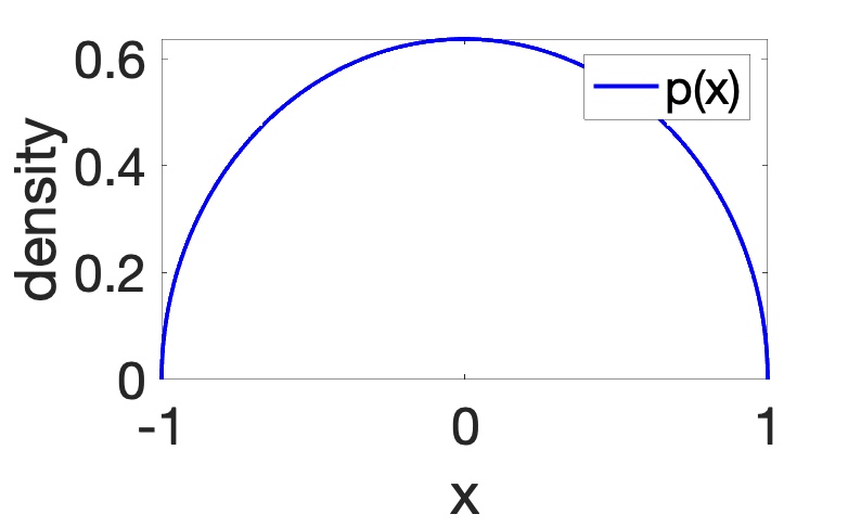
All moments are available in closed form (see end of post), and the Shannon relative entropy is equal to \(D(p\|q) = \int_{-1}^1 \! \frac{2}{\pi} \sqrt{1-x^2} \log \frac{4}{\pi} \sqrt{1-x^2} dx \approx 0.0484\). We can then compute for various values of \(r\), \(D(\Sigma_p \| \Sigma_q)\), which is plotted below.

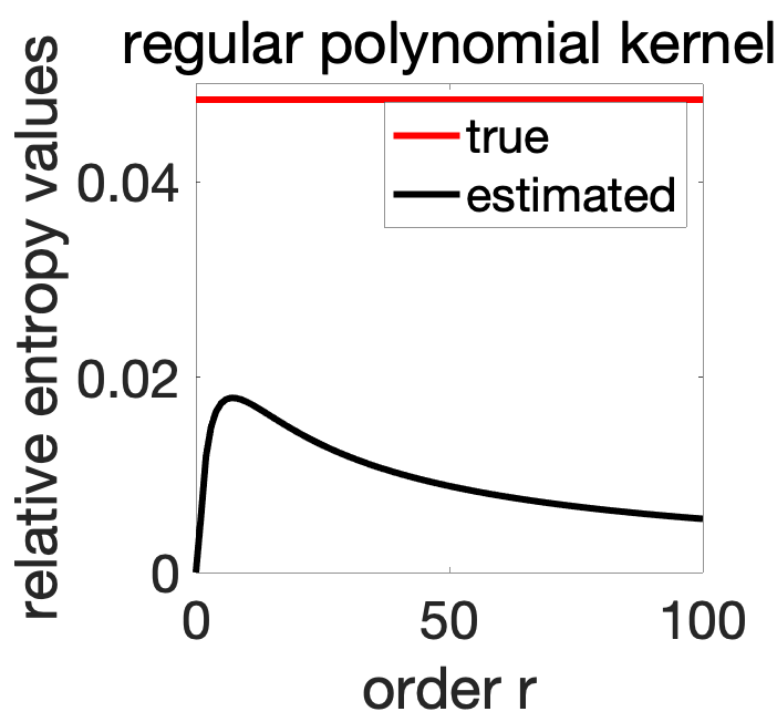
We should hope that the approximation improves as we use more monomials, but this is not the case. As common in kernel methods, the standard polynomial kernel does not have a good behavior. This is partly due to the fact that \(k(x,x) = \big( \frac{1+x^2}{2} \big)^r\) is far from uniform on \([-1,1]\).

Let’s now consider a better polynomial kernel.

Christofell-Darboux kernels. Other polynomial bases could be used as well beyond \(1, X, \dots, X^r\), in particular any basis of polynomials with increasing degrees \(P_0, \dots, P_r\) can be used, in particular polynomials that are orthogonal with respect to a probability distribution on \([-1,1]\), with $$ \varphi(x)_j = \frac{1}{\sqrt{\alpha_r}} P_j(x) \mbox{ and } k(x,y) = \frac{1}{\alpha_r} \sum_{j=0}^r P_j(x) P_j(y),$$ where \(\alpha_r\) is here to ensure that \(k(x,x) \leqslant 1\) on \([-1,1]\). The kernel function \(k(x,y)\) has then itself a simple expression through the Christoffel–Darboux formula, as $$ k(x,y) \propto \frac{P_r(x)P_{r+1}(y)-P_r(y)P_{r+1}(x)}{x-y},$$ with an explicit proportionality constant. For more details on these kernels and their application to data analysis, see [5].

For example, for Chebyshev polynomials, which are orthonormal with respect to the probability measure with density \(\big(\pi \sqrt{1-x^2}\big)^{-1}\) on \([-1,1]\), we have \(P_0 = 1\), \(P_1 = \sqrt{2} X\), and \(P_2 = \sqrt{2}( 2X^2 – 1) \), and more generally, for \(k>0\), \(P_k(\cos \theta) = \sqrt{2}\cos k\theta\). One can then check that for \(x = \cos \theta\) and \(y = \cos \eta\), we have $$k(x,y) = \frac{1}{2} \Big( \frac{ \sin ( 2r+1)( \theta-\eta)/2}{\sin ( \theta-\eta)/2} + \frac{ \sin ( 2r+1)( \theta+\eta)/2}{\sin ( \theta+\eta)/2} \Big).$$ Moreover, we can check that $$ \sup_{x \in \, [-1,1]} k(x,x) = 2r+1, $$ leading to \(\alpha_r = 2r+1\).

As shown below, after computing (still in closed form, see end of the post) \(\Sigma_p\) and \(\Sigma_q\), we can plot the relative entropy, and compare it to the true one. This leads to an improved estimation.

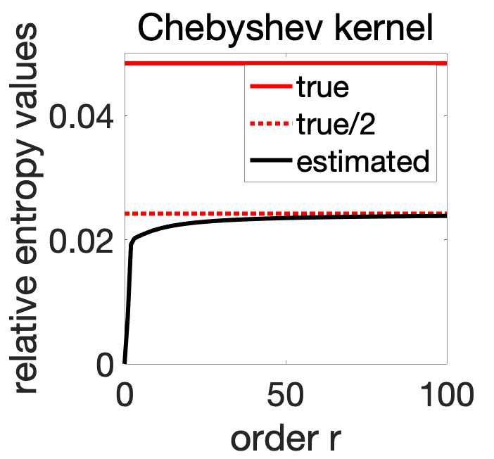
This is better, but still not quite there, and we get in fact convergence to exactly one half of the true relative entropy. The motivated reader will check that the limit of \(k(x,x)\) when \(r \) tends to infinity is \(1/2\) for all \(x \in (-1,1)\), and \(1\), for \(x \in \{-1,1\}\) (that is, the upper-bound of \(1\) is valid, but it is almost surely equal to \(1/2\)). This is where we lose the factor of \(1/2\) in Eq. (1) above.

One key overall insight is that the span of the feature space is not the only important aspect in the approximation, and that some rescalings are better than others (more on this below when optimize with respect to the chosen basis). Given that we end up estimating entropies from moments, it would be clearly interesting to compare with other ways of estimating entropies from moments, such as using asymptotic expansions based on Edgeworth expansions [8].

Fourier series and translation-invariant kernels

We still consider \(\mathcal{X} = [-1,1]\). For a \(2\)-periodic function \(q: \mathbb{R} \to \mathbb{R}\), such that \(q(0) = 1\), with Fourier series \(\hat{q}: \mathbb{Z} \to \mathbb{C}\), we can consider $$k(x,y) = q(x-y) = \sum_{\omega \in \mathcal{Z}} \hat{q}(\omega) e^{i\pi \omega(x-y)}.$$ We can for example take $$q(x) = \frac{\sin ( 2r+1) \pi x/2}{(2r+1)\sin \pi x/2} $$ which corresponds to \(\hat{q}(\omega) = \frac{1}{2r+1} 1_{|\omega| \leqslant r}\), and having $$ \varphi(x)_\omega = \frac{1}{\sqrt{2r+1}} e^{ i\pi \omega x } $$ for \(\omega \in \{-r-1,\dots,r+1\}\) (we consider complex-valued features for simplicity). We refer to this kernel as the Dirichlet kernel.

Link with eigenvalues of Toeplitz matrices. For the specific choice of the Dirichlet kernel, the element of the covariance matrix indexed by \(\omega\) and \(\omega’\) has value \(\int_{-1}^1 e^{i\pi (\omega-\omega’)} dp(x)\), which is the characteristic function of \(p\) evaluated at \(\pi(\omega-\omega’)\). One consequence is that \(\Sigma_p\) is a Toeplitz matrix with constant values across all diagonals. It is then well-known that as \(m\) goes to infinity, the eigenvalues of \(\Sigma_p\) are tending in distribution to \(p\) (see [10]), which provides another proof of good estimation of the entropy in this very particular case.

Note that we could also consider an infinite-dimensional kernel \(q(x) =\Big( 1+ \frac{\sin^2 \pi x/2}{\sinh^2 \sigma}\Big)^{-1}\) which corresponds to \( \hat{q}(\omega) \propto e^{-2\sigma |\omega|}\), where the link with Toeplitz matrices does not apply. See [1] for details.

Increasing number of frequencies. We can then plot the estimation of the same relative entropy as for polynomial kernels, as the number of frequency grows (we can still get the Fourier moments in closed form, see end of post).

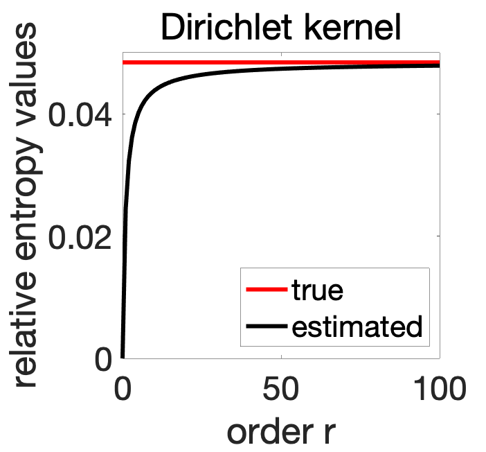
We now see that as the dimension of the feature space grows, we get a perfect estimation of the relative entropy.

This estimation is provably from below, but how far is it? How big \(r\) needs to be?

Upper-bound trough quantum information theory

In order to find a lower-bound \(D(\Sigma_p \| \Sigma_q)\), we cannot rely on Jensen’s inequality, as it is in the wrong direction (this happens a lot!). But here, quantum information theory can come to the rescue.

Using the covariance matrix \(\Sigma\) associated to the uniform distribution \(\tau\) on \(\mathcal{X}\), we consider the PSD matrices \(D(y)\), indexed by \(y \in \mathcal{X}\), equal to $$D(y) = \Sigma^{-1/2} \varphi(y) \varphi(y)^\top \Sigma^{-1/2},$$ for which we have $$\int_{\mathcal{X}} D(y) d\tau(y) =\Sigma^{-1/2} \Big( \int_{\mathcal{X}} \varphi(y) \varphi(y)^\top d\tau(y)\Big)\Sigma^{-1/2} = I. $$ We can now consider, in quantum information theory terms, that each \(D(y)\) corresponds to a measurement that can be applied to a density operator, and that we look at measures obtained from \(p\), as \(\tilde{p}(y) = {\rm tr } ( D(y) \Sigma_p)\), and from \(q\) as \(\tilde{q}(y) = {\rm tr } ( D(y) \Sigma_q)\). This is a proper quantum operation because the matrices \(D(y)\) are PSD and sum to identity.

The monotonicity of the von Neumann entropy with respect to quantum operations [9] applies, and we immediately get $$D(\Sigma_p \| \Sigma_q) \geqslant \int_{\mathcal{X}} \tilde{p}(y) \log \frac{ \tilde{p}(y)}{\tilde{q}(y)} d\tau(y).$$ The lower-bound can be seen as the Shannon relative entropy \(D( \tilde{p} \| \tilde{q} )\) between the distributions with density \(\tilde{p}\) and \(\tilde{q}\) with respect to \(\tau\).

These densities have direct relationships with \(p\) and \(q\). Indeed, we have $$\tilde{p}(y) = {\rm tr } ( D(y) \Sigma_p) = \int_{\mathcal{X}} \big( \varphi(x)^\top \Sigma^{-1/2} \varphi(y) \big)^2 dp(x).$$ Denoting $$h(x,y) = \big( \varphi(x)^\top \Sigma_\tau^{-1/2} \varphi(y) \big)^2,$$ we have \(\int_{\mathcal{X}} h(x,y) d\tau(x) = \| \varphi(y)\|^2\) for all \(y \in \mathcal{X}\), and thus, when the features have unit norms, we can consider \(h\) as a smoothing kernel, and thus \(\tilde{p}\) and \(\tilde{q}\) as smoothed versions of \(p\) and \(q\). Thus, overall we have: $$D(\tilde{p} \| \tilde{q}) \leqslant D(\Sigma_p \| \Sigma_q) \leqslant D(p\|q),$$ and we have sandwitched the kernel relative entropy by Shannon relative entropies.

We can then characterize the error made in estimating the relative entropy by measuring how the smoothing kernel \(h(x,y)\) differs from a Dirac. In [1, Section 4.2], I show how, for metric spaces, the difference between \(D(\tilde{p} \| \tilde{q})\) and \(D({p} \|{q}) \), and thus between \(D(\Sigma_p \| \Sigma_q)\) and \(D(\tilde{p} \| \tilde{q})\), is upperbounded by an explicit function of \(p\) and \(q\), times $$ \sup_{x \in \mathcal{X}} \int_{\mathcal{X}} h(x,y) d(x,y)^2 d\tau(y),$$ which is indeed small when \(h(x,y)\) is closed to a Dirac.

For the Dirichlet kernel presented above, we can show that $$h(x,y) = \frac{1}{4r+2} \bigg( \frac{\sin ( 2r+1) \pi (x-y)/2}{\sin \pi (x-y)/2}\bigg)^2,$$ and that the quantity above characterizing convergence scales as \(1 / (2r+1)\), thus providing an explicit convergence rate. As an illustration, we plot the smoothing kernel at \(y=0\), that is, \(h(x,0)\) in regular scale (left) and log-scale (right), for the Dirichlet kernel above (for which we have unit norm features) for various values of \(r\). We see how it converges to a Dirac as \(r\) grows.

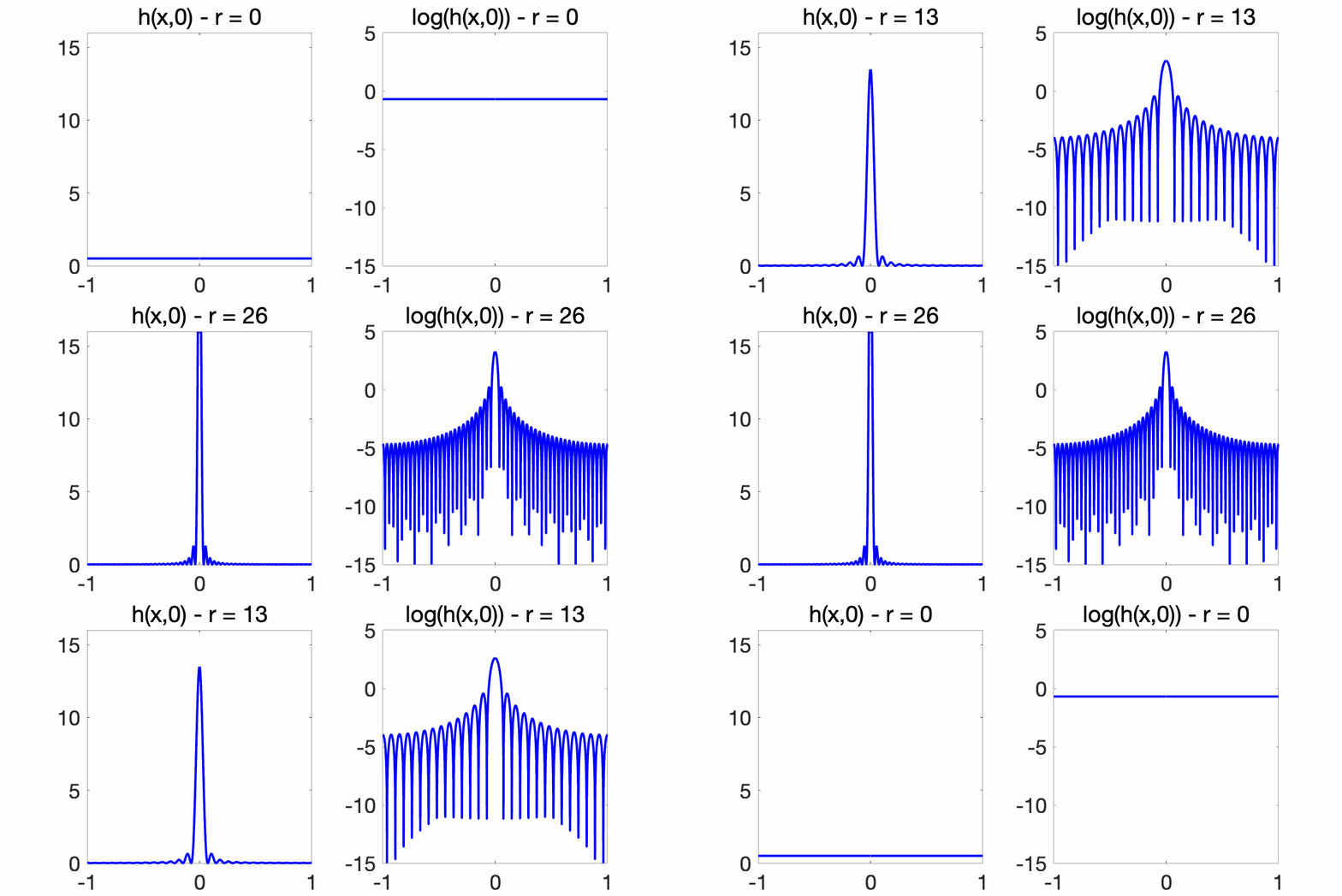
Estimation

Above, we have relied on finite-dimensional feature maps and explicit expectations under \(p\) and \(q\). This is clearly not scalable to generic situations and potentially infinite-dimensional feature spaces. But we can rely here on 30 years of progress in kernel methods.

For simplicity here, we will only estimate the von Neumann entropy \({\rm tr}\big[ \Sigma_p \log \Sigma_p \big]\) from \(n\) independent and identically distributed samples. The natural estimator is \({\rm tr}\big[ \hat{\Sigma}_p \log \hat{\Sigma} _p \big]\), where \(\hat{\Sigma}_p\) and \(\hat{\Sigma}_q\) are empirical covariance matrices (the averages of \(\varphi(x_i) \varphi(x_i)^\top\) over all data points \(x_1,\dots,x_n\)).

In order to compute it efficiently, we can use the usual kernel trick, exactly as used within kernel principal component analysis, and if \(K\) is the \(n \times n\) kernel matrix associated with the \(n\) data points, then the eigenvalues of \(\frac{1}{n} K\) and \(\hat{\Sigma}_p\) are the same, and thus $$ {\rm tr}\big[ \hat{\Sigma}_p \log \hat{\Sigma} _p \big] = {\rm tr}\big[ \big(\frac{1}{n}K \big)\log \big( \frac{1}{n} K \big) \big].$$

In terms of statistical analysis, we refer to [1] where it is shown that the difference between the estimate and the true value is of order \(C / \sqrt{n}\), with an explicit constant \(C\), for a wide range of kernels. Surprisingly, there is no need to add any form of regularization.

Entropy estimation. Together with the approximation result presented above, by letting \(r\) go to infinity for the Dirichlet kernel, we get an estimator of the regular Shannon entropy which is not that bad (see [7] for an optimal one).

Learning representations

As mentioned above for polynomials, a key question is how to choose a feature map \(\varphi: \mathcal{X} \to \mathbb{R}^d\). Given that we have a lower-bound on the relative entropy, it is tempting to try to maximize this lower bound, subject to \(\forall x \in \mathcal{X}\), \(\| \varphi(x)\|^2 \leqslant 1\). The magic is that this is a tractable optimization problem (concave maximization with convex constraints) in the kernel function \((x,y) \mapsto \varphi(x)^\top \varphi(y)\). This is not an obvious result (in fact, I first tried to prove that the von Neumann relative entropy was convex in the kernel, while it is in fact concave). See [1] for the concavity proofs and simple optimization algorithms.

Duality and log-partition functions

Given that our kernel notions of relative entropies are lower bounds on the regular notions, by the traditional convex duality results between maximum entropy and log-partition functions (see, e.g., [11]), we should obtain upper-bounds on log-partition functions. This is exactly what we can get, we simply provide the gist here and refer to [1] for further details.

Given a probability distribution \(q\) on \(\mathcal{X}\) and a function \(f: \mathcal{X} \to \mathbb{R}\), the log-partition function is defined as $$a(f) = \log \bigg( \int_{\mathcal{X}} e^{f(x)} dq(x)\bigg) \tag{2}.$$ It plays a crucial role in probabilistic and statistical inference, and obtaining upper-bounds is instrumental in deriving approximate inference algorithms [11]. A classical convex duality result shows a link with the Shannon relative entropy, as we can express \(a(f)\) as $$a(f) = \sup_{ p\ {\rm probability} \ {\rm measure}} \int_{\mathcal{X}} f(x) dp(x) \ – D( p \| q).$$

Assuming that all features have unit norm, we have \(D(p \|q) \geqslant D(\Sigma_p \| \Sigma_q)\), and thus $$ a(f) \leqslant \sup_{ p \ {\rm probability} \ {\rm measure}} \int_{\mathcal{X}} f(x) dp(x)\ – D(\Sigma_p \| \Sigma_q),$$ which is itself smaller than the supremum over all signed measures with unit mass (thus removing the non-negativity constraint). Therefore, $$ a(f) \leqslant \sup_{ p \ {\rm measure}} \int_{\mathcal{X}} f(x) dp(x)\ – D(\Sigma_p \| \Sigma_q) \tag{3},$$ which can be made computationally tractable in a number of cases.

Conclusion

In this blog post, I tried to exhibit a new link between kernels and information theory, which mostly relies on the convexity properties of von Neumann entropy and a bit of quantum analysis. Clearly, the practical relevance of this link remains to be established, but it opens tractable information theory tools to all types of data on which positive kernels can be defined (essentially all of them), with many potential avenues for future work.

Multivariate modelling. Regular entropies and relative entropies are used extensively in data science, such as for variational inference, but also to characterize various forms of statistical dependences between random variable. It turns out that the new kernel notions allow for this as well, connecting with a classical line of work within kernel methods [12, 13].

Other divergences. I have focused primarily on the link with Shannon relative entropies, but most of the results extend to all \(f\)-divergences. For example, we can get kernel-based lower bounds on the square Hellinger distance, or the \(\chi^2\)-divergences.

Kernel sum-of-squares with a probabilistic twist. As a final note, there is a link between the new notions of kernel entropies with global optimization with kernel sum-of-squares [14]. Indeed, in Eq. (2), if we add a temperature parameter \(\varepsilon\) and define $$a_\varepsilon(f) =\varepsilon \log \bigg( \int_{\mathcal{X}} e^{f(x) / \varepsilon} dq(x) \bigg), $$ then when \(\varepsilon\) tends to zero, \(a_\varepsilon(f) \) tends to \(\sup_{x \in \mathcal{X}} f(x)\). The lower bound from Eq. (3) then becomes $$\sup_{ p \ {\rm measure}} \int_{\mathcal{X}} f(x) dp(x) \ – \varepsilon D(\Sigma_p \| \Sigma_q),$$ which exactly tends to the sum-of-squares relaxation for the optimization problem. Given that for global optimization, smoothness can be leveraged to circumvent the curse of dimensionality, we can imagine something similar for log-partition functions and entropies.

Acknowledgements. I would like to thank Loucas Pillaud-Vivien for proofreading this blog post and making good clarifying suggestions.

References

[1] Francis Bach. Information Theory with Kernel Methods. Technical report, arXiv:2202.08545, 2022.
[2] Brian Kulis, Mátyás A. Sustik, Inderjit S. Dhillon. Low-Rank Kernel Learning with Bregman Matrix Divergences. Journal of Machine Learning Research 10(2):341-376, 2009.
[3] Inderjit S. Dhillon, Joel A. Tropp. Matrix nearness problems with Bregman divergences. SIAM Journal on Matrix Analysis and Applications 29(4):1120-1146, 2008.
[4] Thomas M. Cover and Joy A. Thomas. Elements of Information Theory. John Wiley & Sons, 1999.
[5] Edouard Pauwels, Mihai Putinar, Jean-Bernard Lasserre. Data analysis from empirical moments and the Christoffel function. Foundations of Computational Mathematics 21(1):243-273, 2021.
[6] Ronald De Wolf. A brief introduction to Fourier analysis on the Boolean cube. Theory of Computing, 1:1-20, 2008.
[7] Yanjun Han, Jiantao Jiao, Tsachy Weissman, and Yihong Wu. Optimal rates of entropy estimation
over Lipschitz balls. The Annals of Statistics, 48(6):3228–3250, 2020.
[8] Marc M. Van Hulle. Edgeworth approximation of multivariate differential entropy. Neural computation, 17(9):1903-1910, 2005.
[9] Mark M. Wilde. Quantum Information Theory. Cambridge University Press, 2013.
[10] Robert M. Gray. Toeplitz and Circulant Matrices: A Review. Foundations and Trends in Communications and Information Theory, 2(3):155-239, 2006.
[11] Martin J. Wainwright and Michael I. Jordan. Graphical Models, Exponential Families, and Variational
Inference. Foundations and Trends in Machine Learning, 1(1–2), 1-305, 2008.
[12] Francis Bach and Michael I. Jordan. Kernel independent component analysis. Journal of Machine
Learning Research, 3(Jul):1–48, 2002
[13] Bharath K. Sriperumbudur, Arthur Gretton, Kenji Fukumizu, Bernhard Schölkopf, and Gert R. G.
Lanckriet. Hilbert space embeddings and metrics on probability measures. Journal of Machine Learning Research, 11:1517–1561, 2010.
[14] Alessandro Rudi, Ulysse Marteau-Ferey, and Francis Bach. Finding global minima via kernel approximations. Technical Report 2012.11978, arXiv, 2020

Integrals in closed form

In order to compute in closed form \(\Sigma_p\) for the distribution \(p\) with density on \([-1,1]\) equal to \( \frac{2}{\pi} \sqrt{1-x^2}\), we need to compute some integrals

• Polynomial kernel: we have $$\int_{-1}^1 \frac{2}{\pi} \sqrt{1-x^2}x^{2k} dx = 2^{1-2k} \frac{ ( 2k-1)!}{(k-1)! (k+1)!}.$$
• Chebyshev kernel: we need to compute the integral $$\int_0^{\pi } \frac{2}{\pi} \sin ^2(\theta) \cos^2 k\theta \, d\theta,$$ which is equal to \(1\) for \(k=0\), to \(1/4\) for \(k=1\), and to \(1/2\) for all larger integers. We also need the integral $$\int_0^{\pi } \frac{2}{\pi} \sin ^2(\theta) \cos k\theta \cos(k+2)\theta \, d\theta,$$ which is equal to \(-1/2\) for \(k=0\), and to \(-1/4\) for all larger integers.
• Dirichlet kernel: we have $$ \int_{-1}^1 \frac{2}{\pi} \sqrt{1-x^2} \cos k \pi x dx = \frac{2}{k \pi} J_1(k\pi),$$ where \(J_1\) is the Bessel function of the first kind.