Closed-form dynamics beyond quadratics

Quadratic functions are the workhorse of the analysis of iterative algorithms such as gradient-based optimization. They lead, in discrete and continuous time, to closed-form dynamics that treat all eigensubspaces of the Hessian matrix independently. This leads to simple math for understanding convergence behaviors (maximal step-size, condition number, acceleration, scaling laws for gradient descent or its stochastic version, etc.).

An important success of the optimization field is to have shown that the same behaviors hold for convex functions, where the analysis now relies on Lyapunov functions rather than closed-form computations (see, e.g., this post on automated proofs), with some extensions to non-convex functions, but only regarding convergence to stationary points.

Going (globally) non-convex is of major interest in different fields, including machine learning for neural networks or matrix factorizations. In this post, I try to answer the following question: What are dynamics that lead to closed form or enough of it to get relevant insights?

Over the years, several have emerged, allowing us to give some nice and explicit intuitive results on the global behavior of gradient descent in certain non-convex cases. This blog post is about them. Note that this complements the analysis of diagonal networks from [1, 2] that we described in an earlier post.

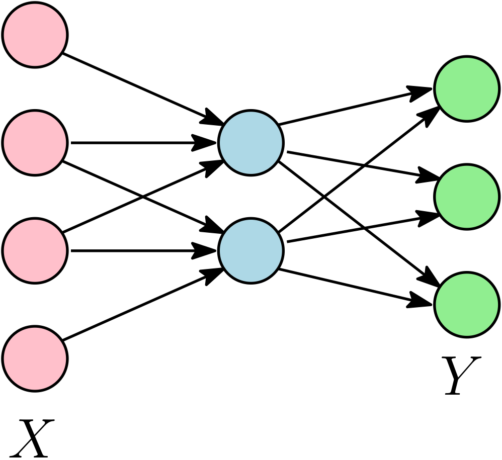
We focus on linear neural networks, with a prediction function \(x \mapsto A_2^\top A_1^\top x\), where \(x \in \mathbb{R}^d\) is the input, \(A_1 \in \mathbb{R}^{d \times m}\) is the matrix of input weights, and \(A_2 \in \mathbb{R}^{m \times k}\) is the matrix of output weights, with an overall weight matrix \(\Theta = A_1 A_2 \in \mathbb{R}^{d \times k}\). This is a linear model corresponding to multi-task / multi-category classification / multi-label supervised problems, or an auto-encoder for unsupervised learning. Clearly, using the parameterization \(\Theta = A_1 A_2\) is not the most efficient for optimization (as we could simply use convex optimization directly on \(\Theta\)), but we use it for understanding non-convex dynamics.

Given data matrices \(Y \in \mathbb{R}^{n \times k}\) and \(X \in \mathbb{R}^{n \times d}\), the empirical risk is $$ L(A_1,A_2) = \frac{1}{2n} \big\| Y – X A_1 A_2 \big\|_{\rm F}^2,$$ where \(\| M \|_{\rm F} = \sqrt{ {\rm tr} (M^\top M)}\) is the Frobenius norm of \(M\).

The gradient flow dynamics are then $$ \left\{ \begin{array}{lcrcr} \dot{A}_1 & = & – \nabla_{A_1} L(A_1,A_2) & = & \frac{1}{n} X^\top ( Y – X A_1 A_2) A_2^\top \\ \dot{A}_2 & = &- \nabla_{A_2} L(A_1,A_2) & = & \frac{1}{n} A_1^\top X^\top ( Y – X A_1 A_2). \\ \end{array} \right.$$

We denote by \(B_1 \in \mathbb{R}^{d \times m}, B_2 \in \mathbb{R}^{m \times k}\) the initialization of the dynamics. As first outlined by [3] and used in most subsequence analyses (e.g., [4, 6, 7]), there is an invariant of the dynamics, as $$\frac{d}{dt} ( A_1^\top A_1 ) = 2 {\rm Sym} \big( A_1^\top \frac{1}{n} X^\top ( Y – X A_1 A_2) A_2^\top \big) = \frac{d}{dt} ( A_2 A_2^\top ), $$ where \({\rm Sym}(M) = \frac{1}{2} ( M + M^\top)\) is the symmetrization of the square matrix \(M\). This implies that \(A_1^\top A_1 – A_2 A_2^\top \in \mathbb{R}^{m \times m}\) is constant along the dynamics. This will allow considerable simplifications (the presence of such invariants is not limited to linear networks, see [16] for a nice detailed account on these conservation laws).

There are several lines of work to go further. I will use a non-chronological presentation and start with the simplest case where singular vectors are aligned, before moving to the real magic first detailed by Kenji Fukumizu in [3].

Aligned initialization and commuting moments

The first set of assumptions that lead to a closed form is, from [4] with \(X^\top X \) proportional to identity, and [5] for this present version:

1. Commuting moments: \(X^\top X\) and \(X^\top YY^\top X\) commute, which is equivalent to aligned singular value decompositions \(C = \frac{1}{n} X^\top Y = U {\rm Diag}(c) V^\top\) and \(\Sigma = \frac{1}{n} X^\top X = U {\rm Diag}(s) U^\top\) for matrices \(U \in \mathbb{R}^{d \times r},V \in \mathbb{R}^{k \times r}\) with orthonormal columns (that is, \(U^\top U = V^\top V = I\)), and \(c,s \in \mathbb{R}_+^r\) non-negative vectors of singular values (this is thus the “economy-size” version of the SVD where \(U\) and \(V\) have the same number of columns). We only need to take \(r\) as big as \(\max \{ {\rm rank}(C), {\rm rank}(\Sigma) \}\). This occurs, for example, when \(X^\top X \propto I\) (whitened data), or for auto-encoders, where \(Y = X\).
2. Aligned initialization: \(B_1 = U {\rm Diag}(b_1) W^\top\) and \(B_2 = W {\rm Diag}(b_2) V^\top\) are the singular value decompositions, with \(W \in \mathbb{R}^{m \times r}\) with orthonormal columns (which implies that we need to assume \(m \geqslant r\)), with singular vectors of \(B_1 B_2 = U {\rm Diag}(b_1 b_2) V^\top\) aligned with the one of \(X^\top Y\).

Note that throughout the blog post, as done just above, multiplication and divisions of the (singular) vectors of the same size will be considered component-wise.

With these assumptions, throughout the dynamics, it turns out that we keep aligned singular vectors, and thus, if \(a_1, a_2\) are the vectors of singular values of \(A_1, A_2\), we get the coupled ODEs: $$ \left\{ \begin{array}{lcr} \dot{a}_1 & = & ( c \, – s a_1 a_2 ) a_2 \\ \dot{a}_2 & = & ( c \, – s a_1 a_2 ) a_1 . \\ \end{array} \right.$$ The invariant mentioned above leads to $$ a_1 a_1 – a_2 a_2 = {\rm cst}.$$ Overall we get the dynamics for \(\theta = a_1 a_2\), $$ \dot{\theta}= ( c \, – s a_1 a_2 ) ( a_1 a_1 + a_2 a_2).$$

If \(b_1 = b_2 = \alpha \) at initialization (for all singular values) with \(\alpha\) a positive scalar, then this remains true throughout the dynamics, and we get $$ \dot{\theta} = 2 ( c \, – s \theta ) \theta, $$ with a closed form dynamics by integration $$\theta = \frac{c}{s} \Big( \frac{e^{2ct} {\alpha^2 }}{\frac{c}{s} – \alpha^2+e^{2ct} {\alpha^2}}\Big) = \frac{1}{ \frac{1}{\alpha^2} e^{-2ct} + \frac{s}{c} ( 1 – e^{-2ct} )}.$$

Insights. We see the sequential learning of each singular values when the initialization scale \(\alpha\) tends to zero, as then we have $$ \theta \sim \frac{1}{ \frac{1}{\alpha^2} e^{-2ct} + \frac{s}{c}},$$ with a sharp jump from \(0\) to \(\frac{c}{s}\), around the time \(\frac{1}{c} \log \frac{1}{\alpha}\).

To prove it, we rescale time as \(t= u \log \frac{1}{\alpha}\) and we get $$\theta = \frac{1}{ \alpha^{2(cu-1)} + \frac{s}{c}},$$ which, with \(u\) fixed, has its \(i\)-th component that converges to \(0\) for \(u < \frac{1}{c_i}\) and to \(c_i / s_i\) for \(u > \frac{1}{c_i}\).

Extension to deeper models. Following [4], we can consider more layers and minimize $$ \frac{1}{2n} \| Y – X A_1 \cdots A_L\|_{\rm F}^2.$$ If at initialization, all singular vectors of all \(A_i\)’s align, then we get dynamics directly on the singular values, and starting from equal values, we get after a few lines $$\dot{\theta} = L (c-s\theta) \theta^{2 – 2/L},$$ which can also be integrated and analyzed. See [4] for details, and [18] for deep linear networks beyond aligned initialization.

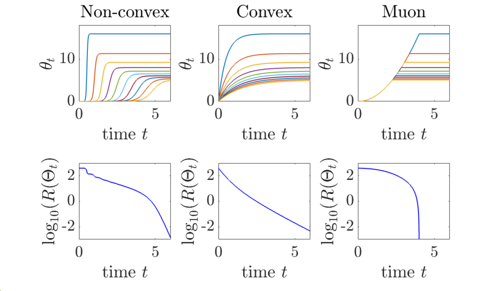
Other dynamics. In this simple case, we can easily compare the dynamics of learning for three common algorithms, which all leads to dynamics on singular values \(\theta\) in this aligned case:

• Gradient descent on \((A_1,A_2)\): As seen above \(\displaystyle \theta = \frac{1}{ \frac{1}{\alpha^2} e^{-2ct} + \frac{s}{c} ( 1 – e^{-2ct} )}\). The singular values \(c\) of \(\frac{1}{n} X^\top Y\) characterize the dynamics, with each singular value appearing one by one when \(\alpha\) is small.
• Gradient descent on \(\Theta = A_1 A_2\) starting from zero (e.g., \(\alpha=0\)): \(\theta = \frac{c}{s} ( 1 – e^{-st})\). The singular values \(s\) of \(\frac{1}{n} X^\top X\) characterize the dynamics.
• Muon: this is the new cool algorithm (“stylé” my kids would say). It corresponds to orthogonalizing the matrix updates, and thus, to do sign descent with vanishing step-size on the singular values, that is, \(\dot{a}_1 = \dot{a}_2 = 1\) until reaching the solution. This leads to \(\theta = \min \{ t^2, c/s\}\), with a conditioning that does not depend on \(s\) or \(c\). No singular values is impacting the dynamics, hence the “automatic” reconditioning, which extends what can be seen for sign descent (see previous post). Note that if we implement Muon directly on \(\Theta\), we would obtain instead \(\theta = \min \{ t, c/s\}\).

Matrix Riccati equation

The second set of assumptions is:

1. White moment matrix: \(\Sigma = \frac{1}{n} X^\top X = I\). Thus, the only data matrix left is \(C = \frac{1}{n} X^\top Y\).
2. Balanced initialization: \(B_1^\top B_1 = B_2 B_2^\top\), which implies that throughout the dynamics, we have \(A_1^\top A_1 = A_2 A_2^\top\) (because of the invariant).

Note that there are no assumptions regarding the alignments of singular vectors at initialization. We also assume that \(m \leqslant r = {\rm rank}(C) \leqslant \min\{d,k\}\). See [17] for closed-form expressions with larger width \(m\).

Then something magical happens, first outlined by Kenji Fukumizu [3], and then further used in several works (e.g., [7, 17, 18]). Defining \(R = { A_1 \choose A_2^\top} \in \mathbb{R}^{(d+k) \times m}\), we have $$R^\top R = A_1^\top A_1 + A_2 A_2^\top = 2A_1^\top A_1 = 2 A_2 A_2^\top,$$ which leads to the rewriting of the dynamics as: $$\dot{R} = \Delta R \, – \frac{1}{2} RR^\top R \mbox{ with } \Delta = \left( \begin{array}{cc} 0 & \!\frac{1}{n}X^\top Y \!\\ \! \frac{1}{n} Y^\top X \! & 0 \end{array} \right)= \left( \begin{array}{cc} 0 & \! C \!\\ \! C^\top \! & 0 \end{array} \right),$$ initialized with \(R_0 = { B_1 \choose B_2^\top} \in \mathbb{R}^{(d+k) \times m}\).

This is now a matrix Riccati equation [8, 9], with a closed form and nice links with several branches of mathematics, such as control (linear-quadratic regulator), probabilistic modelling (Kalman filtering), and machine learning (Oja flow for principal component analysis [10]). In this present post, we will only scratch the surface of this fascinating topic, but a future post will most likely do it justice.

Denoting \(P = RR^\top\), we get $$\dot{P} = \Delta P + P \Delta\, – P^2,$$ and we can then write $$P = NM^{-1}$$ with \(M\) initialized at \(I\) and \(N\) initialized at \(R_0 R_0^\top = { B_1 \choose B_2^\top}{ B_1 \choose B_2^\top}^\top\), and the linear dynamics $$\frac{d}{dt} { M \choose N} = \left( \begin{array}{cc} \! – \Delta \! & \! I \! \\ \! 0 \! & \! \Delta \! \end{array} \right){ M \choose N}.$$ The magical proof (see [10]) is really simple: $$\dot{P} = \dot{N} M^{-1} – N M^{-1} \dot{M} M^{-1} = \Delta N M^{-1} – N M^{-1} ( -\Delta M + N) M^{-1} = \Delta P + P \Delta\, – P^2.$$ This dynamics can be rewritten as $$ \left\{ \begin{array}{rcl} \frac{d}{dt} N & = & \Delta N \\ \frac{d}{dt} ( N\, – 2 \Delta M) & = & – \Delta ( N \, – 2 \Delta M), \end{array} \right.$$ and thus leads to the closed form $$ P = e^{\Delta t} R_0 R_0^\top \Big( e^{-\Delta t} + \frac{e^{\Delta t} – e^{-\Delta t}}{2\Delta } R_0 R_0^\top \Big)^{-1} = e^{\Delta t} R_0 \Big( I + R_0^\top \frac{e^{2\Delta t}-I}{2\Delta } R_0 \Big)^{-1} R_0^\top e^{\Delta t}.$$

We can now analyze this closed-form expression precisely with the following eigenvalue decomposition of \(\Delta\) $$\Delta = \frac{1}{2} { U \choose V} {\rm Diag}(c) { U \choose V}^\top +\frac{1}{2} { U \choose -V} {\rm Diag}(-c) { U \choose -V}^\top,$$ classically obtained for the Jordan-Wielandt matrix \(\Delta\) associated with \(C\) (see an earlier post) with singular value decomposition \(C = U {\rm Diag}(c) V^\top\).

Recovering aligned initialization. We start with aligned initialization (as before, and with the same notations), that is, \(b_1= b_2 =a\). By taking \(B_1 = U {\rm Diag}(a) W^\top\) and \(B_2 = W {\rm Diag}(a) V^\top\), we get \(R_0 = { U \choose V} {\rm Diag}(a) W^\top\), and for any function \(f: \mathbb{R} \to \mathbb{R}\), we have \(f(\Delta) R_0 = { U \choose V} {\rm Diag}(a f(c)) W^\top\), where \(c\) is the vector of singular values of \(C =\frac{1}{n} X^\top Y\), leading to $$P = { U \choose V} {\rm Diag} \Big( \frac{a^2 e^{2 c t}}{ 1 + a^2 \frac{e^{2c t}-1}{c}} \Big){ U \choose V}^\top,$$ which leads to $$ A_1 A_2 = U {\rm Diag} \Big( \frac{a^2 e^{2 c t}}{ 1 + a^2 \frac{e^{2c t}-1}{c}} \Big) V^\top,$$ which is exactly the same as the “aligned” result (OUF!). Note that the aligned initialization only requires that \(C\) and \(\Sigma\) commute, which is weaker than the assumption \(\Sigma =I\) that is made here (but we can go much further below).

Beyond aligned initialization. When \(R_0\) is initialized randomly (and thus with full rank on all subspaces) with balanced initialization and norm proportional to \(\alpha^2\), then, with \(t = u \log \frac{1}{\alpha}\), we also can prove sequential learning of all singular subspaces. More precisely, if \(c_1 > \cdots > c_r\), then, when \(\alpha\) tends to zero (see proof below the reference section):

• If \(u<\frac{1}{c_1}\), \(P \sim 0\). This is the initial phase with no apparent movements, but an alignment of singular vectors, nicely cast as silent alignment by [7].
• When \(u \in ( \frac{1}{c_i}, \frac{1}{c_{i+1}})\) for \(i \in \{1,\dots,m-1\}\), we get \(P \sim C_i\), the optimal rank \(i\) approximation of \(C\).
• When \(u > \frac{1}{c_m}\), \(P \sim C_m\), which is the global minimizer of the cost function.

Note that when \(m = r\), we get \(C_m = C\). Overall, this is exactly sequential learning, with both the singular values and the singular vectors learned from scratch. In the plot below, we see how singular vectors align early in the dynamics when \(\alpha\) is small, while singular values are learned step-by-step.

Conclusion

Overall, we obtain a precise behavior for data with an identity covariance matrix, showing that features (singular vector directions) are learned early on, while their weights (singular values) are learned sequentially. This was done using a balanced initialization (see [11] for an extension beyond balanced initialization and large layer width).

However, this study only applies to linear neural networks (without any non-linear activation function). Extensions to the simplest architectures remain an active area of research (see, e.g., [12] and references therein), with in particular similar early alignment behaviors [13, 14]. In addition, matrix product parameterizations also arise in attention architectures through the product of the key and query matrices. As a result, sequential learning phenomena can also be observed in this setting; see [15] for an analysis of sequential learning in linear attention.

Acknowledgements. I would like to thank Raphaël Berthier, Pierre Marion, Loucas Pillaud-Vivien, and Aditya Varre for proofreading this blog post and making good, clarifying suggestions.

References

[1] Blake Woodworth, Suriya Gunasekar, Jason D. Lee, Edward Moroshko, Pedro Savarese, Itay Golan, Daniel Soudry, Nathan Srebro. Kernel and rich regimes in overparametrized models. Conference on Learning Theory, 2020.
[2] Scott Pesme, Loucas Pillaud-Vivien, and Nicolas Flammarion. Implicit bias of SGD for diagonal linear networks: a provable benefit of stochasticity. Advances in Neural Information Processing Systems, 2021.
[3] Kenji Fukumizu. Effect of batch learning in multilayer neural networks. International Conference on Neural Information Processing, 1998.
[4] Andrew M. Saxe, James L. McClelland, Surya Ganguli. Exact solutions to the nonlinear dynamics of learning in deep linear neural networks. International Conference on Learning Representations, 2014.
[5] Gauthier Gidel, Francis Bach, and Simon Lacoste-Julien. Implicit Regularization of Discrete Gradient Dynamics in Linear Neural Networks. Advances in Neural Information Processing Systems, 2019.
[6] Simon S. Du, Wei Hu, and Jason D. Lee. Algorithmic regularization in learning deep homogeneous models: Layers are automatically balanced. Advances in Neural Information Processing Systems, 2018.
[7] Alexander Atanasov, Blake Bordelon, and Cengiz Pehlevan. Neural Networks as Kernel Learners: The Silent Alignment Effect. International Conference on Learning Representations, 2022.
[8] Vladimír Kučera. A review of the matrix Riccati equation. Kybernetika, 9.1:42-61, 1973.
[9] Richard S. Bucy. Global theory of the Riccati equation. Journal of Computer and System Sciences, 1.4:349-361, 1967.
[10] Wei-Yong Yan, Uwe Helmke, and John B. Moore. Global analysis of Oja’s flow for neural networks. IEEE Transactions on Neural Networks, 5.5:674-683, 1994.
[11] Aditya Vardhan Varre, Maria-Luiza Vladarean, Loucas Pillaud-Vivien, Nicolas Flammarion. On the spectral bias of two-layer linear networks. Advances in Neural Information Processing Systems, 2023.
[12] Alberto Bietti, Joan Bruna, and Loucas Pillaud-Vivien. On learning Gaussian multi-index models with gradient flow. Technical report arXiv:2310.19793, 2023.
[13] Hartmut Maennel, Olivier Bousquet, and Sylvain Gelly. Gradient descent quantizes ReLU network features. Technical report arXiv:1803.08367, 2018.
[14] Etienne Boursier and Nicolas Flammarion. Early alignment in two-layer networks training is a two-edged sword. Journal of Machine Learning Research 26:1-75, 2025.
[15] Yedi Zhang, Aaditya K. Singh, Peter E. Latham, Andrew Saxe. Training Dynamics of In-Context Learning in Linear Attention. International Conference on Machine Learning, 2025.
[16] Sibylle Marcotte, Rémi Gribonval, and Gabriel Peyré. Abide by the law and follow the flow: Conservation laws for gradient flows. Advances in Neural Information Processing Systems, 2023.
[17] Lukas Braun, Clémentine C. J. Dominé, James E. Fitzgerald, Andrew M. Saxe. Exact learning dynamics of deep linear networks with prior knowledge. Advances in Neural Information Processing Systems, 2022.
[18] Sanjeev Arora, Nadav Cohen, Wei Hu, Yuping Luo. Implicit regularization in deep matrix factorization. Advances in Neural Information Processing Systems, 2019.

Proofs

We can rewrite the dynamics as (note that \(\Delta\) is not positive semidefinite) $$ P = \Big( \frac{ 2 \Delta}{1-e^{-2\Delta t}}\Big)^{1/2} H ( H + I)^{-1} \Big( \frac{ 2 \Delta}{1-e^{-2\Delta t}}\Big)^{1/2} ,$$ with $$H = \Big( \frac{e^{2\Delta t}-I}{2\Delta } \Big)^{1/2} R_0 R_0^\top \Big( \frac{e^{2\Delta t}-I}{2\Delta } \Big)^{1/2}.$$ We note that the eigenvalues of \(\Delta\) are singular values of \(C\) as well as their opposite, together with zeros.

The term \(\big( \frac{ 2 \Delta}{1-e^{-2\Delta t}}\big)^{1/2}\) is a spectral function of \(\Delta\) which will set to zero all negative eigenvalues and set to \(( 2 c)^{1/2}\) all positive ones \(c\). We can therefore only consider the positive ones, and consider these terms as identity. Zeros eigenvalues of \(\Delta\) also lead to decay, this time in \(1/t\), and can be discarded as well in the asymptotic analysis.

The term \(\big( \frac{e^{2\Delta t}-I}{2\Delta } \big)^{1/2}\), with strictly positive eigenvalues, is equivalent to \(e^{\Delta t} ( 2 \Delta)^{-1/2}\), and we are faced with studying the dynamics of \(H(I+H)^{-1}\) for \(H = e^{\Delta t} \alpha^2 M e^{\Delta t}\) for \(M = \Delta^{-1} R_0 R_0^\top \Delta^{-1}\) a rank-\(m\) \(r \times r\) matrix, when \(\alpha\) tends to zero. We rewrite \(t = u \log \frac{1}{\alpha}\), and we then have, once in the basis of singular vectors $$H = {\rm Diag}(\alpha^{1-cu}) M {\rm Diag}(\alpha^{1-cu}),$$ with \(N \in \mathbb{R}^{r\times r}\) a rank-\(m\) matrix. We assume \(c_1 > \cdots > c_r\) for simplicity and consider three cases.

Case 1. If \(1- c_i u > 0\) for all \(i\), that is, \(u < 1/c_1\), then the matrix \({\rm Diag}(\alpha^{1-cu}\) goes to zero, and thus \(P\) goes to zero.

Case 2. For \(j \in \{1,\dots,m\}\), and \(u \in [\frac{1}{c_j}, \frac{1}{c_{j+1}}]\), then we have $$H = \left( \begin{array}{cc} D_\infty A D_\infty & D_\infty B D_0 \\ D_0 B^\top D_\infty & D_0 C D_0 \end{array} \right),$$ for a diagonal matrix \(D_\infty\) (of size \(j\)) that goes to infinity and a diagonal matrix \(D_0\) goes to zero. Using \(H (H+I)^{-1} = I – (H+I)^{-1}\) and using Schur complements, we have $$ (H+I)^{-1} = \left( \begin{array}{cc} \bar{A} & \bar{B} \\ \bar{B}^\top & \bar{C} \end{array} \right),$$ with $$\bar{A}^{-1} = I + D_\infty A D_\infty – D_\infty B D_0 ( D_0 C D_0 +I )^{-1}D_0 B^\top D_\infty \sim I + D_\infty A D_\infty,$$ so that \(\bar{A}\) tends to zero (since \(A\) is invertible). We also have $$\bar{C}^{-1} = I + D_0 C D_0 – D_0 B^\top D_\infty ( D_\infty C D_\infty +I )^{-1}D_\infty B D_\infty \sim I,$$ with a similar limit for the off-diagonal block. Therefore \((H+I)^{-1}\) tends to \(\left( \begin{array}{cc} 0 & 0 \\ 0 &I \end{array} \right)\), which leads to the desired result.

Case 3. For \(u > 1/c_m\), using the same formula for \((H+I)^{-1}\), with now \(D_0\) not tending to zero, we can use the fact that \(C = B^\top A^{-1} B\) to obtain the desired limit.