Computer-aided analyses in optimization

In this blog post, I want to illustrate how computers can be great allies in designing (and verifying) convergence proofs for first-order optimization methods. This task can be daunting, and highly non-trivial, but nevertheless usually unavoidable when performing complexity analyses. A notable example is probably the convergence analysis of the stochastic average gradient (SAG) [1], whose original proof was computer assisted.

To this end, we will mostly spend time on what is referred to as performance estimation problems (PEPs), introduced by Yoel Drori and Marc Teboulle [2]. Performance estimation is also closely related to the topic of integral quadratic constraints (IQCs), introduced in the context of optimization by Laurent Lessard, Benjamin Recht and Andrew Packard [3]. In terms of presentations, IQCs leverages control theory, whereas PEPs might seem more natural in the optimization community. This blog post essentially presents PEPs from the point of view of [4], instantiated on a running example.

Overview, motivations

First-order methods for continuous optimization belong to the large panel of algorithms that are usually approached via worst-case analyses. In this context, analyses rely on combining inequalities (that are due to assumptions on the problem classes), in potentially long, non-intuitive, and technical, proofs. For the insiders, those proofs all look very similar. For the outsiders, those proofs all look rather repelling, technical (long pages of chained inequalities), probably not interesting, and like computer codes: usually intuitive mostly for their authors.

In what follows, I want to show how (and why) those proofs are indeed all very similar. On the way, I want to emphasize how those combinations of inequalities are related to the “true essence” of worst-case analyses (which rely on computing worst-case scenarios), and to provide examples on how to constructively obtain them.

We take the stand of illustrating the PEP approach on a single iteration of gradient descent, as it essentially contains all necessary ingredients to understand the methodology in other contexts as well. Certain details of the following text are (probably unavoidably) a bit technical. However, going through the detailed computations is not essential, and the text should contain the necessary ingredients for understanding the essence of the methodology.

Running example: gradient descent

Let us consider a naive, but standard, example: unconstrained convex minimization $$x_\star= \underset{x\in\mathbb{R}^d}{\mathrm{arg min}} f(x)$$with gradient descent: \(x_{k+1}=x_k-\gamma \nabla f(x_k)\). Let us assume \(f(\cdot)\) to be continuously differentiable, to have a \(L\)-Lipschitz gradient (a.k.a., \(L\)-smoothness), and to be \(\mu\)-strongly convex. Those functions satisfy, for all \(x,y\in\mathbb{R}^d\):
– strong convexity, see e.g., [5, Definition 2.1.2]: $$\tag{1}f(x) \geqslant f(y)+\langle{\nabla f(y)}; {x-y}\rangle+\tfrac{\mu}{2} \lVert x-y\rVert^2,$$- smoothness, see e.g., [5, Theorem 2.1.5]: $$\tag{2} f(x) \leqslant f(y)+\langle{\nabla f(y)}; {x-y}\rangle+\tfrac{L}{2}\lVert x-y\rVert^2.$$Let us recall that in the case of twice continuously differentiable functions, smoothness and strong convexity amount to requiring that $$\mu I \preccurlyeq \nabla^2 f(x) \preccurlyeq L I,$$ for some \(0< \mu<L< \infty\) and for all \(x\in\mathbb{R}^d\) (in other words, all eigenvalues of \(\nabla^2 f(x)\) are between \(\mu\) and \(L\)). In what follows, we denote by \(\mathcal{F}_{\mu,L}\) the class of \(L\)-smooth \(\mu\)-strongly convex functions (irrespective of the dimension \(d\)).

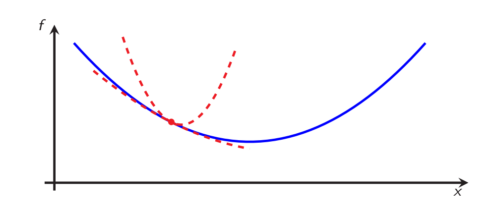
In this context, convergence of gradient descent can be studied in many ways. Here, for the sake of the example, we will do it in terms of two base quantities: distance to optimality \(\lVert x_k-x_\star\rVert\), and function value accuracy \(f(x_k)-f(x_\star)\). There are, of course, infinitely many other possibilities, such as gradient norm \(\rVert \nabla f(x_k)\lVert\), Bregman divergence \(f(x_\star)-f(x_k)-\langle{\nabla f(x_k)};{x_\star-x_k}\rangle\), or even best function value observed throughout the iterations \(\min_{0\leq i\leq k} \{f(x_i)-f(x_\star)\}\): the reader can adapt the lines below for his/her favorite criterion.

For later reference, let us provide another inequality that is known to hold for all \(x,y\in\mathbb{R}^d\) for any \(L\)-smooth \( \mu\)-strongly convex function:
– bound on inner product, see, e.g., [5, Theorem 2.1.11]: $$\langle{\nabla f(x)-\nabla f(y)};{x-y}\rangle \geqslant \tfrac{1}{L+\mu} \lVert{\nabla f(x)-\nabla f(y)}\rVert^2+\tfrac{\mu L}{L+\mu}\lVert{x-y}\rVert^2.\tag{3}$$ In the case \(\mu=0\) this inequality is known as “cocoercivity”. This (perhaps mysterious) inequality happens to play an important role in convergence proofs.

A standard convergence result

Let us start by stating two known results along with their simple proofs (see, e.g., [5, Theorem 2.1.14] or [6, Section 1.4.2, Theorems 2 & 3]):
– convergence in distance: $$\begin{array}{rl} \rVert{x_{k+1}-x_\star}\lVert^2&= \lVert{x_k-x_\star}\rVert^2+\gamma^2\lVert{\nabla f(x_k)}\rVert^2-2\gamma\langle{\nabla f(x_k)};{x_k-x_\star}\rangle \\ \ & \leqslant \left(1-\tfrac{2\gamma L \mu}{L+\mu}\right)\lVert{x_k-x_\star}\rVert^2+\gamma\left(\gamma-\tfrac2{L+\mu}\right)\lVert{\nabla f(x_k)}\rVert^2, \end{array} $$ where the second line follows from smoothness and strong convexity of \(f\) via the bound (3) on the inner product (with \(x=x_k\) and \(y=x_\star\)). For the particular choice \(\gamma=\tfrac2{L+\mu}\), the second term on the right hand side disappears, and we end up with
$$\lVert{x_{k+1}-x_\star}\rVert^2 \leqslant \left(\tfrac{L-\mu}{L+\mu}\right)^2\lVert{x_k-x_\star}\rVert^2,$$ which, following from \(0<\mu<L<\infty\), satisfies \(0< \tfrac{L-\mu}{L+\mu}<1\), hence proving linear convergence of gradient descent in this setup, by recursively applying the previous inequality: $$ \lVert{x_{k}-x_\star}\rVert^2 \leqslant \left(\tfrac{L-\mu}{L+\mu}\right)^{2k}\lVert{x_0-x_\star}\rVert^2.$$ – Convergence in function values: one can simply use the result in distance along with the previous basic inequalities (1) and (2) characterizing smoothness and strong convexity (both with \(y=x_\star\)):
$$f(x_k)-f(x_\star) \leqslant \hspace{-.15cm}\tfrac{L}{2}\hspace{-.1cm}\rVert{x_k-x_\star}\lVert^2 \leqslant \hspace{-.15cm} \tfrac{L}{2}\hspace{-.1cm}\left(\tfrac{L-\mu}{L+\mu}\right)^{\hspace{-.1cm}2k} \rVert{x_0-x_\star}\lVert^2 \leqslant \hspace{-.15cm} \tfrac{L}{\mu}\hspace{-.1cm} \left(\tfrac{L-\mu}{L+\mu}\right)^{\hspace{-.1cm}2k}(f(x_0)-f(x_\star)).$$ It is also possible to directly look for convergence in terms of function values, but it is then usually unclear in the literature what inequalities to use, and I am not aware of any such proof leading to the same rate without the leading \(\tfrac{L}{\mu}\) (except the proof presented below).

At this point, even in this toy example, a few very legitimate questions can be raised:
– can we improve anything? Can gradient descent really behaves like that on this class of functions?
– How could we have guessed the inequality to use, and the shape of the corresponding proof? Obviously, the obscure fact is to arrive to inequality (1). Therefore, is there a principled way for choosing the right inequalities to use, for example for studying convergence in terms of other quantities, such as function values?
– Is this the unique way to arrive to the desired result? If yes, how likely are we to find such proofs for more complicated cases (algorithms and/or function class)?

For the specific step size choice \(\gamma=\tfrac2{L+\mu}\), a partial answer to the first question is obtained by the observation that the rate is actually achieved on the quadratic function
$$f(x)=\tfrac12 \, x^\top \begin{bmatrix}
L & 0\\ 0 & \mu
\end{bmatrix}x.$$ The following lines precisely target the missing answers.

Worst-case analysis through worst-case scenarios

Let us start by rephrasing our goal, and restrict ourselves to the study of a single iteration. We fix our target to finding the smallest possible value of \(\rho\) such that the inequality
$$ \lVert{x_{k+1}-x_\star}\rVert^2 \leqslant \rho^2 \lVert{x_k-x_\star}\rVert^2 $$ is valid for all \(x_k\) and \(x_{k+1}=x_k-\gamma \nabla f(x_k)\) (hence \(\rho\) is a function of \(\gamma\)). In other words, our goal is to solve
$$ \rho^2(\gamma):= \sup \left\{ \frac{\lVert{x_{k+1}-x_\star}\rVert^2}{\lVert{x_k-x_\star}\rVert^2}\, \big|\, f\in\mathcal{F}_{\mu,L},\, x_{k+1}=x_k-\gamma \nabla f(x_k),\, \nabla f(x_\star)=0\right\}.$$
Alternatively, we could be interested in studying convergence in other forms: for function values, we could target to solve the slightly modified problem:
$$ \sup \left\{ \frac{f(x_{k+1})-f(x_\star)}{f(x_{k})-f(x_\star)}\, \big|\, f\in\mathcal{F}_{\mu,L},\, x_{k+1}=x_k-\gamma \nabla f(x_k),\, \nabla f(x_\star)=0 \right\}.$$ It turns out that in both cases, the problem can be solved both numerically to high precision, and analytically, and that the answer is \(\rho^2(\gamma)=\max\{(1-\mu\gamma)^2,(1-L\gamma)^2\}\).

The only thing we did, so far, was to explicitly reformulate the problem of finding the best (smallest) convergence rate as the problem of finding the worst-case scenario, nothing more. In what follows, some parts might become slightly technical, but the overall idea is only to reformulate this problem of finding the worst-case scenarios, for solving it.

Dealing with an infinite-dimensional variable: the function \(f\)

The first observation is that the problem of computing \(\rho\) is stated as an infinite-dimensional optimization problem: we are looking for the worst possible problem instance (a function \(f\) and an initial point \(x_k\)) within a predefined class of problems. The first step we take to work around this is to reformulate it in the following equivalent form (note that we maximize also over the dimension \(d\)—we discuss later how to remove it):
$$\begin{array}{rl} \rho^2:= \underset{f,\, x_k,\,x_\star,\, g_k,\,d}{\sup} &\displaystyle \frac{\lVert{x_{k}-\gamma g_k-x_\star}\rVert^2}{\lVert{x_k-x_\star}\rVert^2}\\
\text{s.t. } & \exists f\in\mathcal{F}_{\mu,L}:\, g_k= \nabla f(x_k),\, 0=\nabla f(x_\star).
\end{array}$$
This problem intrinsically does not look better (it contains an existence constraint), but it allows using mathematical tools which are referred to as interpolation, or extension, theorems [4, 7, 8]. The problem is depicted on Figure 2:

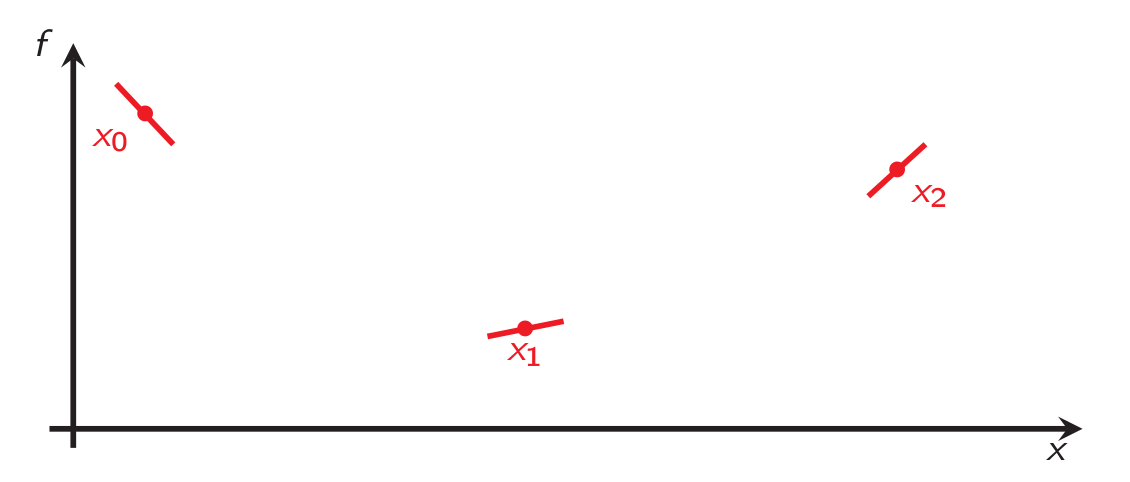
It turns out that convex interpolation (that is, neglecting smoothness and strong convexity) is actually rather simple:

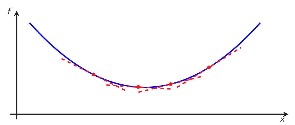
• given a convex function and an index set \(I\), any set of samples \(\{(x_i,g_i,f_i)\}_{i\in I}\) of the form \(\{(\text{coordinate}, \text{(sub)gradient}, \text{function value})\}\)) satisfies, for all \(i,j\in I\): $$f_i \geqslant f_j+\langle g_j; x_i-x_j\rangle,$$ by definition of subgradient, as illustrated on Figure 3.

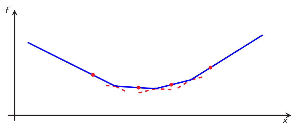
• In the other direction, given a set of triplets \(\{(x_i,g_i,f_i)\}_{i\in I}\) satisfying the previous inequality for all pairs \(i,j\in I\), one can simply recover a convex function by the following construction: $$f(x)=\underset{i\in I}{\max}\{ f_i+\langle g_i;x-x_i\rangle\},$$ which is depicted on Figure 4.

• Formally, the reasoning allows arriving to the following “convex interpolation” (or “convex extension”) result, where we denote the set of (closed, proper) convex functions by \(\mathcal{F}_{0,\infty}\) (to be understood as \(L\)-smooth \(\mu\)-strongly convex functions with \(\mu=0\) and \(L=\infty\)): $$\begin{array}{c}\exists f\in\mathcal{F}_{0,\infty}: \, g_k\in\partial f(x_k) \text{ and } f_k=f(x_k) \ \ \forall k\in I\\ \Leftrightarrow\\ f_i \geqslant f_j+\langle{g_j};{x_i-x_j}\rangle\quad \forall i,j\in I,\end{array}$$ where \(\partial f(x)\) denotes the subdifferential of \(f\) at \(x\).

In the next section, we use a similar interpolation result for taking smoothness and strong convexity into account. The result is a bit more technical, but follows from similar constructions as those for convex interpolation—the main difference being that the interpolation is done on the Fenchel conjugate instead, in order to incorporate smoothness, see [4, Section 2].

Reformulation through convex interpolation

Back to the problem of computing worst-case scenarios, we can now reformulate the existence constraint exactly using the following result (see [4, Theorem 4]): let \(I\) be a finite index set and let \( S=\{(x_i,g_i,f_i)\}_{i\in I}\) be a set of triplets, then
$$\begin{array}{c}\exists f\in\mathcal{F}_{\mu,L}: \, g_i=\nabla f(x_i) \text{ and } f_i=f(x_i) \text{ for all } i\in I\\ \Leftrightarrow\\ f_i \geqslant f_j+\langle{g_j};{x_i-x_j}\rangle+\frac{1}{2L}\lVert{g_i-g_j}\rVert^2+\frac{\mu}{2(1-\mu/L)}\lVert{x_i-x_j-\frac{{1}}{L}(g_i-g_j)}\rVert^2 \,\,\, \forall i,j\in I.\end{array}$$ Therefore, the previous problem can be reformulated as (recalling that \(g_\star=0\))
$$ \begin{array}{rl} \underset{{f_k,\,f_\star,\, x_k,\,x_\star,\, g_k,\,d}} {\sup}&\displaystyle\frac{\rVert{x_{k}-\gamma g_k-x_\star}\lVert^2}{\rVert{x_k-x_\star}\lVert^2}\\
\text{s.t. } & f_\star \geqslant f_k+\langle{g_k};{x_\star-x_k}\rangle+\frac{1}{2L}\lVert{g_k}\rVert^2+\frac{\mu}{2(1-\mu/L)}\lVert{x_k-x_\star-\frac{{1}}{L}g_k}\rVert^2\\
& f_k \geqslant f_\star+\frac{1}{2L}\lVert{g_k}\rVert^2+\frac{\mu}{2(1-\mu/L)}\lVert{x_k-x_\star-\frac{{1}}{L}g_k}\rVert^2.
\end{array}$$

Quadratic reformulation

The next step is to remove the ratio appearing in the objective function, which we do via an homogeneity argument, as follows.

Starting from a feasible point, scale \(x_k,\,x_\star,g_k\) by some \(\alpha>0\) and \(f_k,\,f_\star\) by \(\alpha^2\) and observe it does not change the value of the objective, while still being a feasible point. Therefore, the problem can be reformulated as a nonconvex QCQP (quadratically constrained quadratic program): $$ \begin{array}{rl} \underset{{f_k,\,f_\star,\, x_k,\,x_\star,\, g_k,\,d}} {\sup}&\displaystyle{\rVert{x_{k}-\gamma g_k-x_\star}\lVert^2}\\
\text{s.t. } & f_\star \geqslant f_k+\langle{g_k};{x_\star-x_k}\rangle+\frac{1}{2L}\lVert{g_k}\rVert^2+\frac{\mu}{2(1-\mu/L)}\lVert{x_k-x_\star-\frac{{1}}{L}g_k}\rVert^2\\
& f_k \geqslant f_\star+\frac{1}{2L}\lVert{g_k}\rVert^2+\frac{\mu}{2(1-\mu/L)}\lVert{x_k-x_\star-\frac{{1}}{L}g_k}\rVert^2\\ &{\rVert{x_k-x_\star}\lVert^2} \leqslant 1,
\end{array}$$ which is quadratic in \(x_k\), \(x_\star\) and \(g_k\), and linear in \(f_\star\) and \(f_k\). Actually, in the current form, nonconvexity comes from the term “\(\langle{g_k};{x_\star-x_k}\rangle\)” in the second constraint (and from the objective, due to maximization). It turns out that this problem can be reformulated losslessly using semidefinite programming (this is due to the maximization over \(d\), as commented at the end of the next section).

Semidefinite reformulation

At the end of this section, we will be able to compute, numerically, the values of the rate \(\rho^2(\gamma)\) for given values of the parameters \(\mu,\,L\), and \(\gamma\).

The last step in the reformulation goes as follows: the previous problem can be reformulated as a semidefinite program, as it is linear in terms of the entries of the following Gram matrix
$$G = \begin{pmatrix}
\lVert{x_k-x_\star}\rVert^2 & \langle{g_k};{x_k-x_\star}\rangle \\ \langle{g_k};{x_k-x_\star}\rangle & \lVert{g_k}\rVert^2
\end{pmatrix}\succcurlyeq 0,$$ and in terms of the function values \(f_k\) and \(f_\star\). From those variables, one reformulate the previous problem as $$\begin{array}{rl} \underset{f_k,\,f_\star,\, G\succeq 0}{\sup} \, &{\mathrm{Tr} (A_\text{num} G)}\\
\text{s.t. } & f_k-f_\star+\mathrm{Tr} (A_1 G)\leqslant 0\\
& f_\star-f_k+\mathrm{Tr} (A_2 G)\leqslant 0 \\
&\mathrm{Tr} (A_\text{denom} G) \leqslant 1,\end{array}$$ which is a gentle semidefinite program where we picked matrices \(A_{\text{num}}\), \(A_{\text{denom}}\), \(A_1\) and \(A_2\) for encoding the previous terms. That is, we choose those matrices such that
$$\begin{array}{rl}
\mathrm{Tr}(A_{\text{denom}} G)&=\lVert{x_k-x_\star}\rVert^2,\\ \mathrm{Tr}(A_{\text{num}} G)&=\lVert{x_k-\gamma g_k-x_\star}\rVert^2,\\ \mathrm{Tr}(A_1G)&=\langle{g_k};{x_\star-x_k}\rangle+\frac{1}{2L}\lVert{g_k}\rVert^2+\frac{\mu}{2(1-\mu/L)}\lVert{x_k-x_\star-\frac{{1}}{L}g_k}\rVert^2,\\ \mathrm{Tr}(A_2G)&=\tfrac{1}{2L}\lVert g_k\rVert^2+\tfrac{\mu}{2(1-\mu/L)}\lVert x_k-x_\star-\tfrac1L g_k\rVert^2.\end{array}$$ One possibility is to choose \(A_{\text{num}}\), \(A_{\text{denom}}\), \(A_1\) and \(A_2\) as symmetric matrices, as follows: $$\begin{array}{cc}
A_{\text{denom}}=\begin{pmatrix} 1 & 0\\ 0 & 0 \end{pmatrix}, & A_{\text{num}}=\begin{pmatrix} 1 & -\gamma\\ -\gamma & \gamma^2 \end{pmatrix}, \\ A_1=\begin{pmatrix}\tfrac{\mu}{2(1-\mu/L)} & -\tfrac12-\tfrac{\mu}{2(L-\mu)} \\ -\tfrac12-\tfrac{\mu}{2(L-\mu)} & \tfrac{1}{2L}+\tfrac{\mu}{2L(L-\mu)}\end{pmatrix}, & A_2=\begin{pmatrix}\tfrac{\mu}{2(1-\mu/L)} & -\tfrac{\mu}{2(L-\mu)} \\ -\tfrac{\mu}{2(L-\mu)} & \tfrac{1}{2L}+\tfrac{\mu}{2L(L-\mu)} \end{pmatrix}.\end{array}$$

All those steps can be carried out in the exact same way for the problem of computing the convergence rate for function values, reaching a similar problem with \(6\) inequality constraints instead—because interpolation conditions have to be imposed on all pairs of points in a set of \(3\) points: \(x_k\), \(x_{k+1}\) and \(x_\star\), instead of only \(2\) for the distance problem. The objective function is then \(f_{k+1}-f_\star\), the de-homogenization constraint (arising from the denominator of the objective function) is \(f_{k}-f_\star \leqslant 1\), and the Gram matrix is \(3\times 3\):
$$G=\begin{pmatrix}
\lVert{x_k-x_\star}\rVert^2 & \langle{g_k};{x_k-x_\star}\rangle& \langle{g_{k+1}};{x_k-x_\star}\rangle\\ \langle{g_k};{x_k-x_\star}\rangle & \lVert{g_k}\rVert^2 & \langle{g_k};{g_{k+1}}\rangle \\
\langle{g_{k+1}};{x_k-x_\star}\rangle & \langle{g_{k+1}};{g_k}\rangle & \lVert{g_{k+1}}\rVert^2
\end{pmatrix}\succcurlyeq 0, $$ and the function values variables are \(f_k\), \(f_{k+1}\) and \(f_\star\).

We provide the numerical optimal values of those semidefinite programs on Figure 5 for both convergence in distances and in function values.

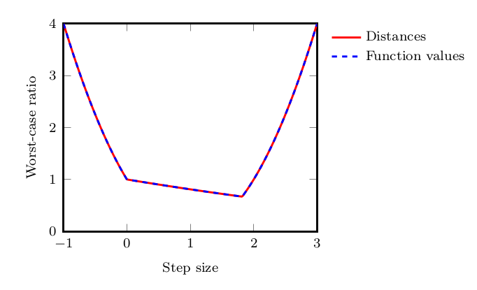
As a conclusion for this section, let us note that we showed how to compute the “best” rates that are dimension independent. In general, requiring the iterates and gradient (e.g., \(x_k\) and \(g_k\) for the problem in terms of distance, and \(x_k\), \(g_k\) and \(g_{k+1}\) for function values, and potentially more vectors when dealing with more complex settings) to lie in \(\mathbb{R}^d\) is equivalent to adding a rank constraint in the SDP.

Duality between worst-case scenarios and combinations of inequalities

Any feasible point to the previous SDP corresponds to a lower bound: a sampled version of a potentially difficult function for gradient descent. If we want to find upper bounds on the rate, a natural way to proceed is to go to the dual side of the previous SDPs, where any feasible point will naturally correspond to an upper bound on the convergence rate (by weak duality). As the primal problems were SDPs, their Lagrangian duals are SDPs as well. Let us associate one multiplier per constraint: $$ \begin{array}{rl}
f_k-f_\star+\mathrm{Tr} (A_1 G)\leqslant 0&:\lambda_1\\
f_\star-f_k+\mathrm{Tr} (A_2 G)\leqslant 0&:\lambda_2\\
\mathrm{Tr}(A_\text{denom} G) \leqslant 1&: \tau.
\end{array}$$The dual is then
$$\begin{array}{rl}
\underset{\tau,\,\lambda_1,\,\lambda_2}{\min} & \, \tau \\
\text{s.t. } & \lambda_1=\lambda_2,\\
& S:=A_\text{num}-\tau A_\text{denom}-\lambda_1A_1-\lambda_2A_2 \preccurlyeq 0,\\
&\tau,\lambda_1,\lambda_2 \geqslant 0.
\end{array}$$ Hence, by weak duality, any feasible point to this last SDP corresponds to an upper bound on the rate: \(\tau \geqslant \rho^2\). A mere rephrasing of weak duality can be obtained through the following reasoning: assume we received some feasible \(\tau,\lambda_1,\lambda_2\) (and hence \(\lambda_1=\lambda_2\) and a corresponding \(S\preccurlyeq 0\)), we then get, for any primal feasible \(G\succcurlyeq0\):
$$\begin{array}{rl}\mathrm{Tr}(SG)&=\mathrm{Tr}(A_{\text{num}}G)-\tau\mathrm{Tr}(A_{\text{denom}}G)-\lambda_1\mathrm{Tr}(A_1G)-\lambda_2\mathrm{Tr}(A_2G)\\&=\lVert x_{k+1}-x_\star\rVert^2-\tau\lVert x_{k}-x_\star\rVert^2\\ \,&\,\,\,-\lambda_1[ f_k-f_\star+\langle{g_k};{x_\star-x_k}\rangle+\frac{1}{2L}\lVert{g_k}\rVert^2+\frac{\mu}{2(1-\mu/L)}\lVert{x_k-x_\star-\frac{{1}}{L}g_k}\rVert^2]\\ &\,\,\,-\lambda_2 [f_\star-f_k+\frac{1}{2L}\lVert{g_k}\rVert^2+\frac{\mu}{2(1-\mu/L)}\lVert{x_k-x_\star-\frac{{1}}{L}g_k}\rVert^2]\\ &\geqslant \lVert x_{k+1}-x_\star\rVert^2-\tau\lVert x_{k}-x_\star\rVert^2, \end{array}$$ where the first equality follows from the definition of \(S\), the second equality corresponds to the definitions of \(A_{\text{num}}\), \(A_{\text{denom}}\), \(A_1\) and \(A_2\), and the last inequality follows from the sign of the interpolation inequalities (constraints in the primal) for any primal feasible point. Hence, we indeed have that any feasible \(\tau\) corresponds to a valid upper bound on the convergence rate, as $$S\preccurlyeq 0 \,\,\Rightarrow \,\, \mathrm{Tr}(SG)\leqslant 0\,\,\Rightarrow \lVert x_{k+1}-x_\star\rVert^2-\tau\lVert x_{k}-x_\star\rVert^2\leqslant 0.$$ In order to obtain analytical proofs, we therefore need to find analytical dual feasible points, and numerics can of course help in this process! Let’s look at what the optimal dual solutions look like for our two running examples.

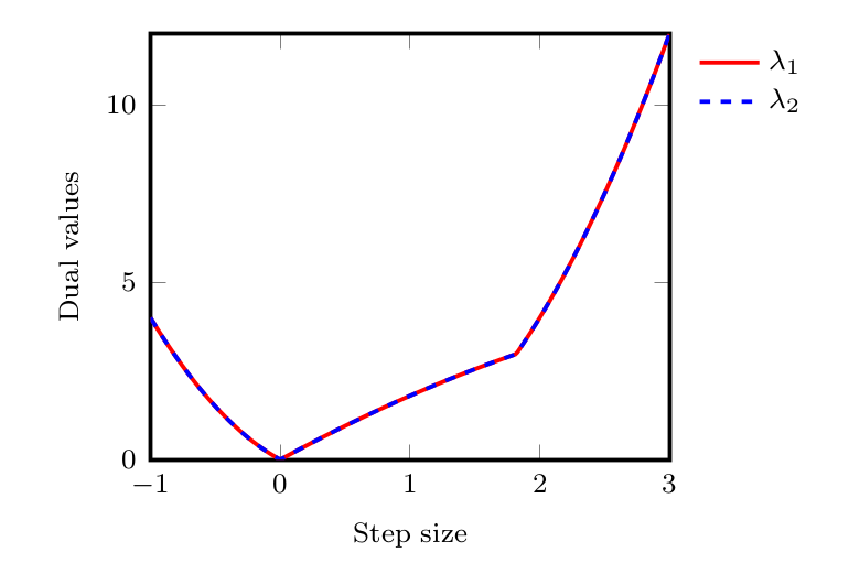
• in Figure 6, we provide the numerical values for \(\lambda_1\) and \(\lambda_2\) for the distance problem.

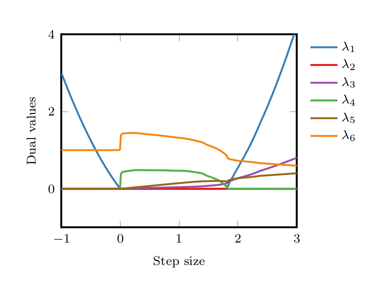
• For function values, the SDP is slightly more complicated, as more inequalities are involved (6 interpolation inequalities). We provide raw numerical values for the six multipliers in Figure 7.

For those who want a bit more details, here are a few additional pointers:

• Strong duality holds—a way to prove it is to show that there exists a Slater point in the primal, see e.g., [4, Theorem 6]—, and hence primal and dual optimal values match.
• There might be different ways to optimaly combine the interpolation inequalities for proving the desired results. In other words: dual optimal solutions are often not unique—which is, in fact, quite a good news: I am sure nobody want to find the analytical version of the multipliers provided in Figure 7.
• It is often possible to simplify the proofs by using fewer, or weaker, inequalities. This might lead to ”cleaner” results, typically (but not always) at the cost of ”weaker” rates. This was done for designing the proof for function values, later in this text.

Combinations of inequalities: same proofs without SDPs

So far, we showed that computing convergence rates can be done in a very principled way. To this end, one can solve semidefinite programs—which may have arbitrarily complicated analytical solutions. Here, I want to emphasize that the process of verifying a solution can be quite different to that of finding a solution. Put in other words, although the dual certificates (a.k.a., the proofs) might have been found by solving SDPs, they can be formulated in ways that do not require the reader to know anything about the PEP methodology, nor on any SDP material, for verifying them. This fact might actually not be very surprising to the reader, as many proofs arising in the first-order optimization literature actually “only consists” in linear combinations of (quadratic) inequalities. On the one hand, those proofs can be seen as feasible points to “dual SDPs”, although generally not explicitely proved as such. On the other hand, proofs arising from the SDPs might therefore be expected to be writable without any explicit reference to semidefinite programing and performance estimation problems.

In what follows, we provide the proofs for gradient descent, using the previous numerical inspiration, but without explicitly relying on any semidefinite program. The reader is not expected to verify any of those computations, as our goal is rather to emphasize that the principles underlying both proofs are exactly the same: reformulating linear combinations of inequalities.

For both proofs below, we limit ourselves to the step size regime \(0\leq \gamma \leq \tfrac{2}{L+\mu}\), and we prove that, in this regime, \(\rho(\gamma)=(1-\gamma\mu)\)—actually we only proof the upper bounds, but one can easily verify that they are tight on simple quadratic functions. The complete proofs (for the proximal gradient method), can be found in [11].

Example 1: distance to optimality

Recall the notations: \(g_k:=\nabla f(x_k)\), \(f_k:= f(x_k)\), \(g_\star:=\nabla f(x_\star)\), and \(f_\star:= f(x_\star)\).

For distance to optimality, sum the following inequalities with their corresponding weights: $$\begin{array}{r} f_\star \geqslant f_k+\langle{g_k};{x_\star-x_k}\rangle+\frac{1}{2L}\lVert{g_k-g_\star}\rVert^2+\frac{\mu}{2(1-\mu/L)}\lVert{x_k-x_\star-\frac{{1}}{L}(g_k-g_\star)}\rVert^2 :\lambda_1, \\ f_k \geqslant f_\star+\langle{g_\star};{x_k-x_\star}\rangle+\frac{1}{2L}\lVert{g_k-g_\star}\rVert^2+\frac{\mu}{2(1-\mu/L)}\lVert{x_k-x_\star-\frac{{1}}{L}(g_k-g_\star)}\rVert^2:\lambda_2. \end{array}$$ We use the following values for the multipliers: \(\lambda_1=\lambda_2=2\gamma\rho(\gamma) \geqslant 0\) (see Figure 6).

After appropriate substitutions of \(g_\star\), \(x_{k+1}\), and \(\rho(\gamma)\), using respectively \(g_\star=0\), \(x_{k+1}=x_k-\gamma g_k\) and \(\rho(\gamma)=(1-\gamma\mu)\), and with little effort, one can check that the previous weighted sum of inequalities can be written in the form: $$ \begin{array}{rl} \lVert{x_{k+1}-x_\star}\rVert^2 \leqslant & \left(1-\gamma \mu \right)^2\lVert{x_{k}-x_\star}\rVert^2 -\frac{\gamma(2-\gamma (L+\mu))}{L-\mu} \lVert{\mu {(x_k -x_\star)} – g_k}\rVert^2. \end{array}$$ This statement can be checked simply by expanding both expressions (i.e., the weighted sum and its reformulation) and verifying that all terms indeed match.

Finally, using $$\gamma(2-\gamma (L+\mu)) \geqslant 0, \text{ and } L-\mu \geqslant 0,$$ which are nonnegative by assumptions on the values of \(L\in(0,\infty)\), \(\mu\in (0,L)\) and \(\gamma\in(0,2/(L+\mu))\), we arrive to the desired $$ \lVert{x_{k+1}-x_\star}\rVert^2 \leqslant \left(1-\gamma \mu \right)^2\lVert{x_{k}-x_\star}\rVert^2.$$

Note that, by using \(\lambda_1=\lambda_2\), the weighted sum exactly corresponds to the (scaled by a positive constant) inequality introduced in the early stage of this note for studying distance to optimality. However, the resulting expression is tight for all values of the step size here, whereas it was only tight for \(\gamma=2/(L+\mu)\) earlier, due to a different choice of weights!

The curious reader might wonder how to find such a reformulation. Actually, back in terms of SDPs, and using the expressions for the multipliers, it simply corresponds to $$\mathrm{Tr}(SG)=-\frac{\gamma(2-\gamma (L+\mu))}{L-\mu} \lVert{\mu {(x_k -x_\star)} – g_k}\rVert^2.$$ In the example below, the reformulation is a bit more tricky—as \(\mathrm{Tr}(SG)\) has two nonnegative terms, which were simply obtained by doing an analytical Cholesky factorization of the term \(\mathrm{Tr}(SG)\)—, but the idea is exactly the same.

Example 2: function values

For function values, we combine the following inequalities after multiplication with their respective coefficients:

$$\scriptsize \begin{array}{lr} f_k \geqslant f_{k+1}+\langle{g_{k+1}};{x_k-x_{k+1}}\rangle+\frac{1}{2L}\lVert{g_k-g_{k+1}}\rVert^2+\frac{\mu}{2(1-\mu/L)}\lVert{x_k-x_{k+1}-\frac{1}{L}(g_k-g_{k+1})}\rVert^2 &:\lambda_1,\\
f_\star \geqslant f_k+\langle{g_k};{x_\star-x_k}\rangle+\frac{1}{2L}\lVert{g_k-g_\star}\rVert^2+\frac{\mu}{2(1-\mu/L)}\lVert{x_k-x_\star-\frac{1}{L}(g_k-g_\star)}\rVert^2 &:\lambda_2, \\
f_\star \geqslant f_{k+1}+\langle{g_{k+1}};{x_\star-x_{k+1}}\rangle+\frac{1}{2L}\lVert{g_\star-g_{k+1}}\rVert^2+\frac{\mu}{2(1-\mu/L)}\lVert{x_\star-x_{k+1}-\frac{1}{L}(g_\star-g_{k+1})}\rVert^2 &:\lambda_3. \end{array}$$ We use the following multipliers \(\lambda_1=\rho(\gamma)\), \(\lambda_2=(1-\rho(\gamma))\rho(\gamma)\), and \(\lambda_3=1-\rho(\gamma)\) (obtained by greedily trying to set different combinations of multipliers to \(0\) in the SDP—see Figure 7 for the values without such simplifications).

Again, after appropriate substitutions of \(g_\star\), \(x_{k+1}\), and \(\rho(\gamma)\), using respectively \(g_\star=0\), \(x_{k+1}=x_k-\gamma g_k\) and \(\rho(\gamma)=(1-\gamma\mu)\), we obtain that the weighted sum of inequalities can be reformulated exactly as $$ \begin{array}{rl} f(x_{k+1})-f_\star \leqslant &\left(1-\gamma \mu\right)^2 \left(f(x_k)-f_\star\right)\\&-\frac{1}{2 (L-\mu)}\lVert \nabla f(x_{k+1})-(1-\gamma (L+\mu))\nabla f(x_k) +\gamma \mu L (x_\star-x_k)\rVert^2\\
&-\frac{\gamma L(2- \gamma (L+\mu))}{2 (L-\mu )}\lVert \nabla f(x_k)+\mu (x_\star-x_k)\rVert^2.\end{array}$$ Again, this statement can be checked simply by expanding both expressions (i.e., the weighted sum and its reformulation), and verifying that all terms match. The desired conclusion $$ f(x_{k+1})-f_\star \leqslant \left(1-\gamma \mu\right)^2 \left(f(x_k)-f_\star\right), $$ follows from the signs of the leading coefficients: \(\gamma(2-\gamma (L+\mu)) \geqslant 0\), and \(L-\mu \geqslant 0\).

To go further

Before finishing, let us mention that we only dealt with linear convergence through a single iteration of gradient descent.

There are quite a few ways to handle both more iterations and sublinear convergence rates. Using SDPs, probably the most natural approach is to directly incorporate several iterations in the problem by studying, for example, ratios of the form $$\sup_{f\in\mathcal{F}_{\mu,L},\, x_0} \frac{f(x_{N})-f_\star}{\lVert x_0-x_\star\rVert^2}. $$ This type of approach was used in the work of Drori and Teboulle [2] and in most consecutive PEP-related works: it has the advantage of providing comfortable “non-improvable results” [4, 12] (by providing matching lower bounds) for any given \(N\), but requires solving larger and larger SDPs. Alternatively, simpler proofs can often be obtained through the use of Lyapunov (or potential) functions—i.e., study a single iteration to produce recursable inequalities; a nice introduction is provided in [13]. This idea can be exploited in PEPs [14] by enforcing the proofs to have a certain structure. Those principles are also at the heart of the related approach using integral quadratic constraints [3, 15].

Take-home message and conclusions

The overall message of this note is that first-order methods can often be studied directly using the definition of their “worst-cases” (i.e., by trying to find worst-case scenarios), along with their dual counterparts (linear combinations of inequalities), by translating them into semidefinite programs.

What we saw might look like an overkill for studying gradient descent. However, as long as we deal with Euclidean spaces, the same approach actually works beyond this simple case. In particular, the same technique applies to first-order methods performing explicit, projected, proximal, conditional, and inexact (sub)gradient steps [12].

Finally, let us mention a few previous works illustrating that the use of such computer-assisted proofs allowed obtaining results that are apparently too complicated for us to find bare-handed—even in apparently simple contexts. Reasonable examples include the direct proof for convergence rates in function values [11] presented above, but also proofs arising in the context of optimized numerical schemes [2, 16, 17, 18]—in particular [18] presents a method for minimizing the gradient norm at the last iterate, in smooth convex minimization—, in the context of monotone inclusions [19], and even for more general fixed-point problems (e.g., for Halpern iterations [20]).

Toolbox

The PErformance EStimation TOolbox (PESTO) [21, see Github] allows a quick access to the methodology without worrying about details of semidefinite reformulations. The toolbox contains many examples (about 50) in different settings, and include progresses on the approach, and results, by other groups (which are much more thoroughly referenced in the user guide). In particular, we included standard classes of functions and operators, along with examples for analyzing recent optimized methods.

References

[1] Mark Schmidt, Nicolas Le Roux, Francis Bach. Minimizing finite sums with the stochastic average gradient. Mathematical Programming, 162(1-2), 83-112, 2017.
[2] Yoel Drori, Marc Teboulle. Performance of first-order methods for smooth convex minimization: a novel approach. Mathematical Programming, 145(1-2), 451-482, 2014.
[3] Laurent Lessard, Benjamin Recht, Andrew Packard. Analysis and design of optimization algorithms via integral quadratic constraints. SIAM Journal on Optimization, 26(1), 57-95, 2016.
[4] Adrien Taylor, Julien Hendrickx, François Glineur. Smooth strongly convex interpolation and exact worst-case performance of first-order methods. Mathematical Programming, 161(1-2), 307-345, 2017.
[5] Yurii Nesterov. Introductory Lectures on Convex Optimization : a Basic Course. Applied optimization. Kluwer Academic Publishing, 2004.
[6] Boris Polyak. Introduction to Optimization. Optimization Software New York, 1987.
[7] Daniel Azagra, Carlos Mudarra. An extension theorem for convex functions of class \(C^{1,1}\) on Hilbert spaces. Journal of Mathematical Analysis and Applications, 446(2):1167–1182, 2017.
[8] Aris Daniilidis, Mounir Haddou, Erwan Le Gruyer, Olivier Ley. Explicit formulas for \(C^{1,1}\) Glaeser-Whitney extensions of 1-Taylor fields in Hilbert spaces. Proceedings of the American Mathematical Society, 146(10):4487–4495, 2018.
[9] Johan Löfberg. YALMIP : A toolbox for modeling and optimization in MATLAB. Proceedings of the CACSD Conference, 2004.
[10] APS Mosek. The MOSEK optimization software. Online at http://www.mosek.com, 54, 2010.
[11] Adrien Taylor, Julien Hendrickx, François Glineur. Exact worst-case convergence rates of the proximal gradient method for composite convex minimization. Journal of Optimization Theory and Applications, vol. 178, no 2, p. 455-476, 2018.
[12] Adrien Taylor, Julien Hendrickx, François Glineur. Exact worst-case performance of first-order methods for composite convex optimization. SIAM Journal on Optimization, vol. 27, no 3, p. 1283-1313, 2017.
[13] Nikhil Bansal, Anupam Gupta. Potential-Function Proofs for Gradient Methods. Theory of Computing, 15(1), 1-32, 2019.
[14] Adrien Taylor, Francis Bach. Stochastic first-order methods: non-asymptotic and computer-aided analyses via potential functions, Proceedings of the 32nd Conference on Learning Theory (COLT), 99:2934-2992, 2019.
[15] Bin Hu, Laurent Lessard. Dissipativity theory for Nesterov’s accelerated method, Proceedings of the 34th International Conference on Machine Learning, 70:1549-1557, 2017.
[16] Yoel Drori, Marc Teboulle. An optimal variant of Kelley’s cutting-plane method. Mathematical Programming 160.1-2: 321-351, 2016.
[17] Donghwan Kim, Jeffrey Fessler. Optimized first-order methods for smooth convex minimization, Mathematical programming, 159(1-2), 81-107, 2016.
[18] Donghwan Kim, Jeffrey Fessler. Optimizing the efficiency of first-order methods for decreasing the gradient of smooth convex functions, preprint arXiv:1803.06600, 2018.
[19] Ernest Ryu, Adrien Taylor, Carolina Bergeling, Pontus Giselsson. Operator splitting performance estimation: Tight contraction factors and optimal parameter selection, SIAM Journal on Optimization (to appear), 2020.
[20] Felix Lieder. On the convergence rate of the Halpern-iteration. Technical Report, 2019.
[21] Adrien Taylor, Julien Hendrickx, François Glineur. Performance estimation toolbox (PESTO): automated worst-case analysis of first-order optimization methods, Proceedings of the 56th Annual Conference on Decision and Control (CDC), pp. 1278-1283, 2017.