In optimization, acceleration is the art of modifying an algorithm in order to obtain faster convergence. Building accelerations and explaining their performance have been the subject of a countless number of publications, see [2] for a review. In this blog post, we give a vignette of these discussions on a minimal but challenging example, Nesterov acceleration. We introduce and illustrate different frameworks to understand and design acceleration techniques: the discrete framework based on iterations, the continuous-time framework, and the recent continuized framework that we proposed in [1].
First, let us describe the setting we use. Let \(f:\mathbb{R}^d \to \mathbb{R}\) be a convex and differentiable function, that we seek to minimize. We assume that \(f\) is \(L\)-smooth, i.e., $$\forall x,y \in \mathbb{R}^d, \qquad f(y) \leq f(x) + \langle \nabla f(x), y-x \rangle + \frac{L}{2} \Vert y-x \Vert^2 \, , $$ and that it is \(\mu\)-strongly convex for some \(\mu > 0\), i.e., $$\forall x,y \in \mathbb{R}^d, \qquad f(y) \geq f(x) + \langle \nabla f(x), y-x \rangle + \frac{\mu}{2} \Vert y-x \Vert^2 \, .$$We had already made these assumptions in a previous blog post on computer-aided analyses in optimization. In this setting, the function \(f\) has a unique minimizer that we denote \(x_*\).
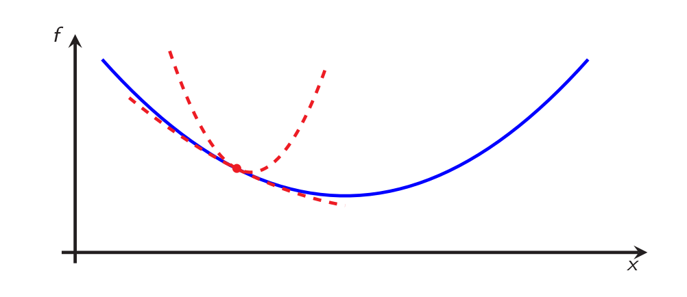
In this figure, the blue function \(f\) is \(L\)-smooth and \(\mu\)-strongly convex: it is possible to create global upper and lower quadratic bounds from every \(x \in \mathbb{R}^d\) with respective curvatures \(L\) and \(\mu\).
Of course, smoothness and strong convexity are not the only assumptions under which acceleration is studied (see [2] for a larger variety of accelerations). In particular, in [1], these is a discussion similar to the one of this blog post in the case where strong convexity is not assumed.
Discrete-time acceleration
The basic algorithm for minimizing \(f\) is gradient descent: we start from an initial guess \(x_0 \in \mathbb{R}^d\) and iterate $$x_{k+1} = x_k \, – \gamma \nabla f(x_k) \, ,$$where \(\gamma\) is a step size.
Let us show how this performs on an example in dimension \(d=2\). In the plot below, the thin curves represent the level sets of the function \(f\). With a slight abuse of notation, we denote \(x_1\) and \(x_2\) the coordinates of the vector \(x \in \mathbb{R}^2\).
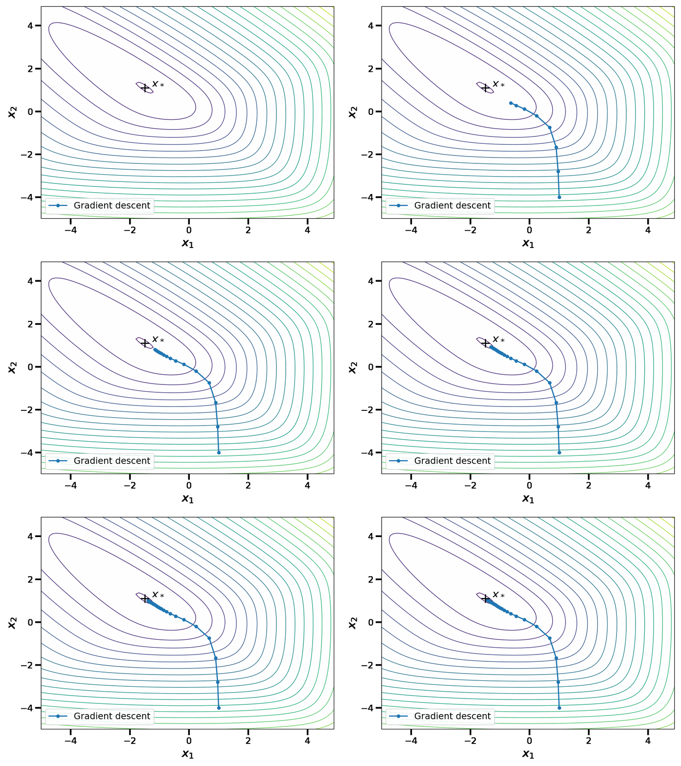
When \(\gamma \leq \frac{1}{L}\), we have the linear convergence rate $$f(x_k) \, – f(x_*) \leq \frac{L}{2} \Vert x_0 \, – x_* \Vert^2 (1-\gamma \mu)^k \, ,$$see [3, Theorem 2.1.15] for instance. This upper bound is minimized at \(\gamma = \frac{1}{L}\), leading to a \(O\big( \left( 1\, – \frac{\mu}{L} \right)^k \big)\) convergence rate. Although this convergence rate is linear, it can be slow when the condition number \(\frac{L}{\mu} \) is large.
To tackle this issue, Nesterov [3] proposed an alternative algorithm: $$\begin{aligned}
&y_k = x_k + \frac{\sqrt{\gamma\mu}}{1 + \sqrt{\gamma\mu}}(z_k-x_k) \, , \\ &x_{k+1} = y_k \, – \gamma \nabla f(y_k) \, , \\ &z_{k+1} = z_k + \sqrt{\gamma\mu}(y_k-z_k) \, – \sqrt{\frac{\gamma}{\mu}}\nabla f(y_k ) \, . \end{aligned}$$

Nesterov proved the following convergence bound for his algorithm: if \(\gamma \leq \frac{1}{L}\), $$f (x_k) \, – f(x_*) \leq \left(f(x_0) \, – f(x_*) + \frac{\mu}{2} \Vert z_0 \, – x_* \Vert^2 \right) \left(1\, – \sqrt{\gamma\mu}\right)^k \, .$$ Again, this upper bound is minimized at \(\gamma = \frac{1}{L}\); this leads to a \(O\left( \left( 1 \, – \sqrt{\frac{\mu}{L}} \right)^k \right)\) convergence rate. The acceleration lies in this new square root dependence in the condition number, that enables significant speed-ups in practice. To show this, let us compare the sequence \(x_k\) of Nesterov acceleration with gradient descent.
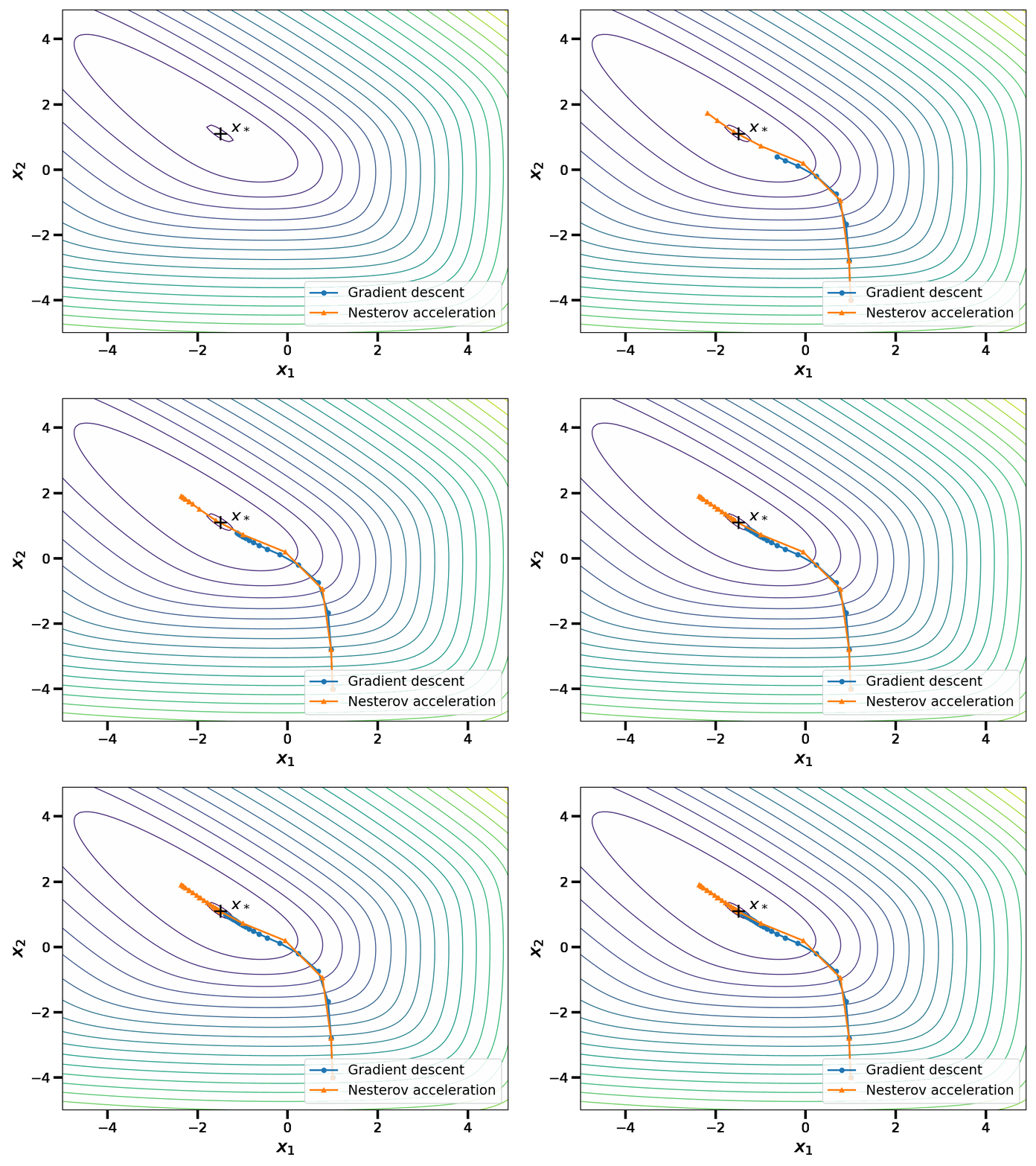
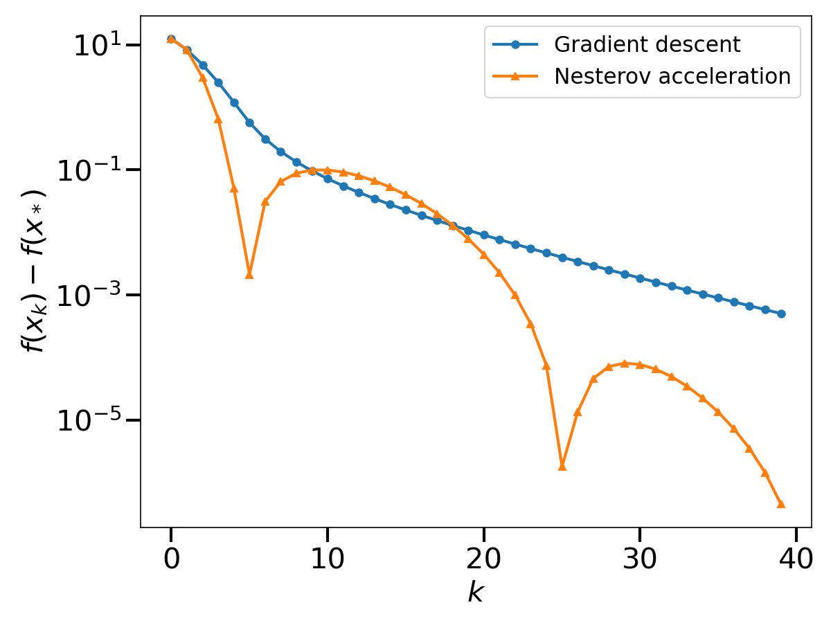
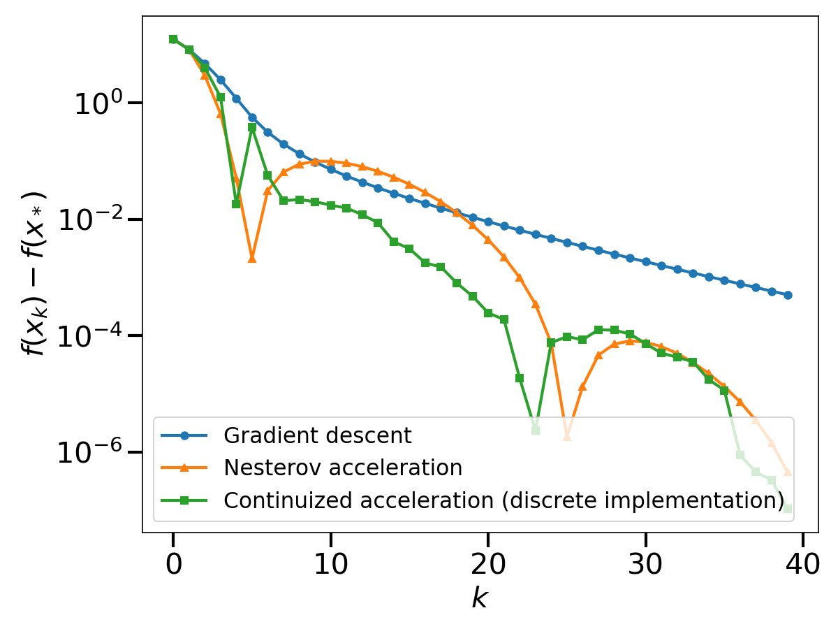
We observe that the asymptotic performance of Nesterov acceleration is much better. Of course, comparing the two algorithms in terms of the iteration number \(k\) is unfair to gradient descent, as the complexity per iteration of Nesterov acceleration is higher. However, as suggested by the theoretical convergence bound, the speed-up provided by Nesterov acceleration is largely worth the additional complexity per iteration on badly conditioned problems.
From a high-level perspective, Nesterov acceleration iterates over several variables, alternating between gradient steps (always with respect to the gradient at \(y_k\)) and mixing steps, where the running value of a variable is replaced by a linear combination of the other variables. However, the precise way gradient and mixing steps are coupled is rather mysterious, and the improved convergence bound relies heavily on the detailed structure of the iterations.
Only an inspection of the proof of the convergence bound [2,3] can provide a rigorous understanding of Nesterov acceleration and its performance. Many works contributed to interpret and motivate the iteration [11-15]. In this blog post, we try to give some high-level intuitions through the continuous and continuized points of view on Nesterov acceleration.
Continuous-time acceleration
Continuous-time approaches propose to gain insights on the above algorithms through their limit as the stepsize \(\gamma\) vanishes [4,10]. This was already the subject of a previous blog post. In this approach, one needs to rescale the iterate number \(k\) as \(\gamma \to 0\) in order to obtain a non-degenerate limit.
For instance, to study gradient descent, we define a rescaled time variable \(t = \gamma k \in \mathbb{R}_{\geq 0}\) and the reparametrized iterates \(X(t) = X(\gamma k) = x_k\). Then for small \(\gamma\), $$\frac{dX}{dt}(t) \approx \frac{X(t+\gamma)-X(t)}{\gamma} = \frac{x_{t/\gamma+1}-x_{t/\gamma}}{\gamma} = \, – \nabla f(x_{t/\gamma}) = \, – \nabla f(X(t)) \, .$$In the limit \(\gamma \to 0\), the approximation of the derivative becomes exact and this gives the gradient flow equation $$\frac{dX}{dt}(t) = \, – \nabla f(X(t)) \, .$$

Note that in the simulation above, the gradient descents are aligned with the gradient flow in terms of their common time parameter \(t = \gamma k\). However, as the stepsize \(\gamma\) is not the same in the two gradient descents, the number of iterations is also not the same.
In [4,5], a similar limit is taken for the iterates \(x_k\) of Nesterov acceleration. As the computations are a bit lengthy, let us simply state the result. Define a rescaled time variable \(t = \sqrt{\gamma} k \in \mathbb{R}_{\geq 0}\) and the reparametrized iterates \(X(t) = X(\sqrt{\gamma} k ) = x_k\). As \(\gamma \to 0\), \(X\) satisfies the ordinary differential equation (ODE) $$ \frac{d^2X}{dt^2}(t) + 2\sqrt{\mu} \frac{dX}{dt}(t) = \, – \nabla f(X(t)) \, .$$
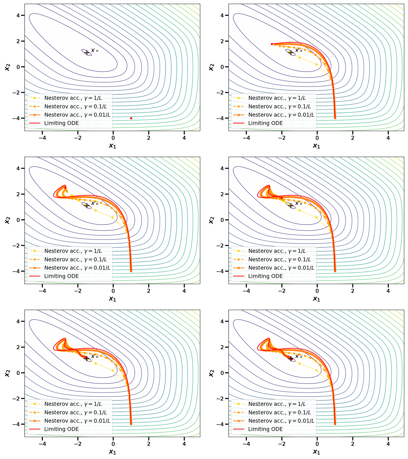
At this point, it is tempting to try to overlap the last two plots in order to compare the gradient flow with the limiting ODE for Nesterov acceleration. However, this can not be done as the notion of time \(t\) is not the same in both cases. The gradient flow is obtained at the limit of gradient descent with \(t_1 = \gamma k\); meanwhile Nesterov acceleration has a continuous limit in the scaling \(t_2 = \sqrt{\gamma} k\). For a small stepsize \(\gamma\), \(t_2\) is an order of magnitude larger than \(t_1\); this confirms that Nesterov acceleration is indeed an acceleration.
The precise ODE obtained in the limit of Nesterov acceleration gives insights on the mechanism underlying acceleration. It is a second-order ODE, while the gradient flow is a first-order ODE. The gradient flow represents the movement of a particle rolling on the graph of \(f\), with no inertia. Meanwhile, the ODE for Nesterov acceleration also represents the movement of a particle rolling on the graph of \(f\), but with inertia and with a friction coefficient proportional to \(\sqrt{\mu}\). This comforts the high-level idea that acceleration is achieved by ”giving inertia to the iterates”.
However, the continuous perspective on acceleration comes with important limitations. First, as illustrated in the plots, the continuous limits appear in a computationally inefficient limit of small stepsizes. However, the rates of convergence of the discrete algorithms depend on their ability to be stable while using large stepsizes; this aspect can not be apprehended in the continuous limit.
Relatedly, the continuous limits are not algorithms by themselves; they need to be discretized to be implemented. The discretization of the accelerated ODE could lead to Nesterov acceleration, but also to multiple other algorithms including Polyak’s heavy ball method (see [6] or [2, Section 2.3.3]), another algorithm that is not as stable on non-quadratic strongly convex functions. Said differently, the continuous limit is unable to discriminate two discrete algorithms with different performances. However, it should be noted that this limitation was adressed in [5] by considering other ODEs that approximate the discrete algorithms at a higher-order when \(\gamma \to 0\).
In the next section, we present the so-called “continuized” version of Nesterov acceleration, a joint work [1] with Mathieu Even, Francis Bach, Nicolas Flammarion, Hadrien Hendrikx, Pierre Gaillard, Laurent Massoulié, Adrien Taylor and myself. It is defined in continuous time, but it does not correspond to a limit where \(\gamma \to 0\). Furthermore, it does not need to be approximated to be implemented in discrete time.
Continuized acceleration
The continuized acceleration is composed of two variables \(x_t\), \(z_t\) indexed by a continuous time \(t \geq 0\), that are continuously mixing and that take gradient steps at random times. More precisely, let \(T_1, T_2, T_3, \dots \geq 0\) be random times such that \(T_1, T_2-T_1, T_3-T_2, \dots\) are independent identically distributed (i.i.d.), of distribution exponential with rate \(1\). The exponential distribution is a classical distribution which has a special memoryless property; in our case of rate \(1\), it is the distribution with density \(\exp(-t)\). Below, we show five realizations of the random times \(T_1, T_2, T_3, \dots\), between \(t=0\) and \(t = 10\):


By convention, we choose that our stochastic processes \(t \mapsto x_t\), \(t \mapsto z_t\) are “càdlàg” almost surely, i.e., right continuous with well-defined left-limits \(x_{t-}\), \(z_{t-}\) at all points \(t\). At random times \(T_1, T_2, \dots\), our sequences take gradient steps $$\begin{aligned} x_{T_k} &= x_{T_k-} – \gamma \nabla f (x_{T_k-}) \, , \\z_{T_k} &= z_{T_k-} – \sqrt{\frac{\gamma}{\mu}} \nabla f (x_{T_k-}) \, . \end{aligned}$$Because of the memoryless property of the exponential distribution, in a infinitesimal time interval \([t, t+dt]\), the variables take gradients steps with probability \(dt\), independently of the past.
Between these random times, the variables mix through a linear, translation-invariant, ODE $$\begin{aligned}&dx_t = \sqrt{\gamma\mu} (z_t \, – x_t) dt \, , \\&dz_t = \sqrt{\gamma\mu} (x_t \, – z_t) dt \, .\end{aligned}$$Following the notation of stochastic calculus, we can write the process more compactly. Denote \(dN(t) = \sum_{k\geq 1} \delta_{T_k}(dt)\) the Poisson point measure; it is the sum of Dirac masses at the random times \(T_1, T_2, \dots\). Then we write
$$\begin{aligned}
dx_t &= \sqrt{\gamma\mu} (z_t \, – x_t) dt \, – \gamma \nabla f(x_t) dN(t) \, , \\
dz_t &= \sqrt{\gamma\mu} (x_t \, – z_t) dt- \sqrt{\frac{\gamma}{\mu}} \nabla f(x_t) dN(t) \, .
\end{aligned}$$This should be understood as detailed above: the first component of these equations is an evolution with respect to the Lebesgue measure, thus a continuous flow; the second component is an evolution with respect to a discrete measure; when the time \(t\) hits a Dirac mass of the measure \(dN(t)\), then we take discrete jumps. This gives a continuous-time random process; we show one realization below.
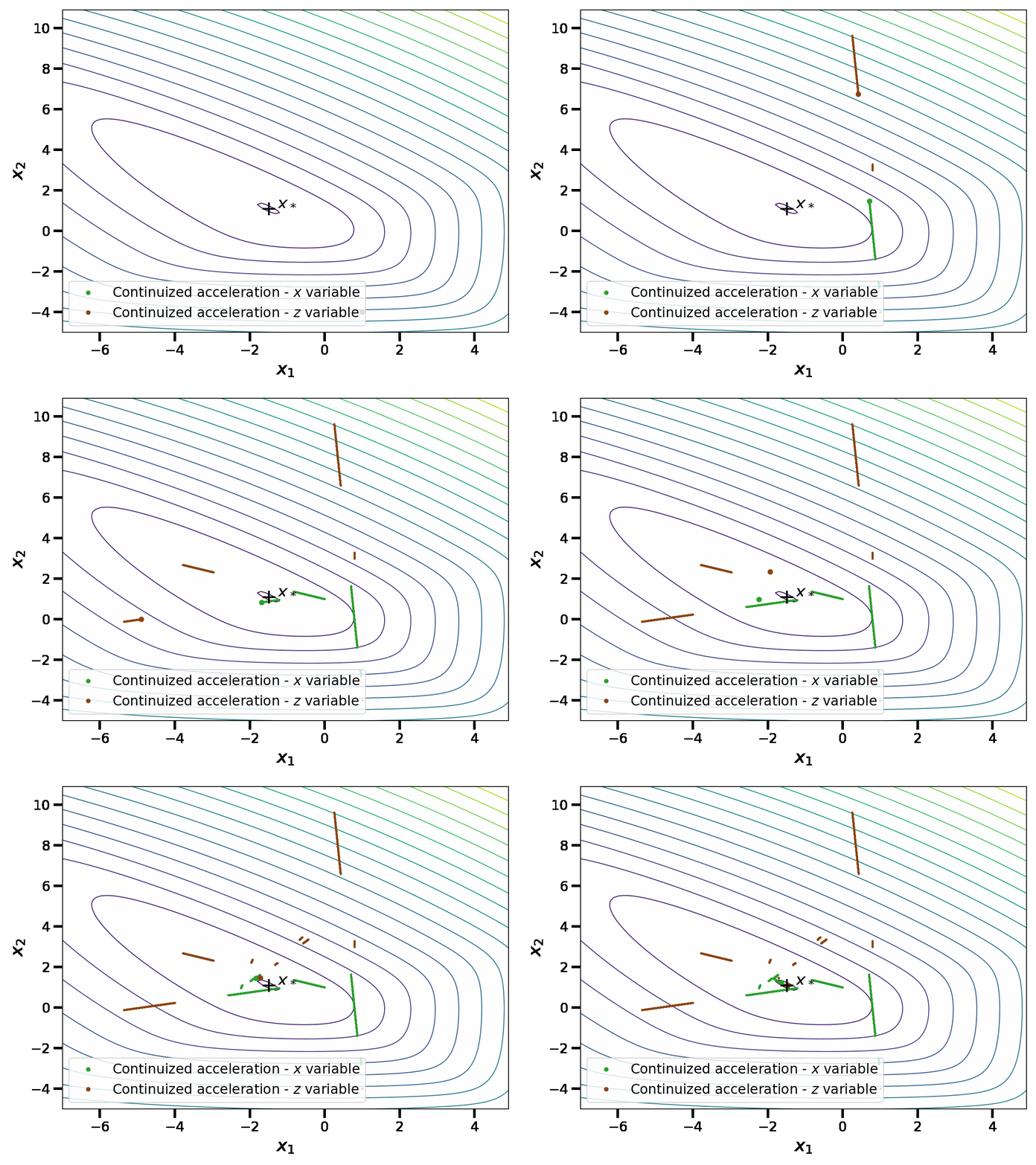
In this simulation, we see similarities with the discrete acceleration of Nesterov. However, the process is now random and in continuous time. We comment this comparison in detail in the rest of the blog post.
In [1], we proved the following convergence bound for this process: if \(\gamma \leq \frac{1}{L}\), $$\mathbb{E} f(x_t) \, – f(x_*) \leq \left(f(x_0) \, – f(x_*) + \frac{\mu}{2} \Vert z_0 \, – x_* \Vert^2 \right) \exp\left( – \sqrt{\gamma \mu} t \right) \, .$$Note the similarity with the bound proved by Nesterov for the discrete acceleration. In fact, the proof through Lyapunov techniques is essentially the same. In the continuized acceleration, the main difference is that we have a statement in expectation over the sampling of the Poisson point measure.
In summary, we observe from the bounds and the simulation that the discrete and continuized accelerations behave similarly. The continuized acceleration is more involved as it is a random process with ODE components and jumps. Why would one prefer the continuized acceleration? Can we discretize the continuized acceleration easily?
In the next section, we explain why the discretization of the continuized acceleration is not a problem. But before that, let us propose high-level answers to the first question.
First, from a Markov chain indexed by a discrete time index \(k\), one can associate the so-called continuized Markov chain, indexed by a continuous time \(t\), that makes transition with the same Markov kernel, but at random times, with independent exponential time intervals [8]. This terminology motivated the name of the continuized acceleration in [1]. The continuized Markov chain is appreciated for its continuous time parameter \(t\), for instance because it enables to use differential calculus. Still, the continuized Markov chain keeps many properties of the original Markov chain; similarly the continuized acceleration is arguably simpler to analyze, while performing similarly to Nesterov acceleration.
Second, processes that alternate randomly are generally simpler to analyze that those that alternate in cycles. For instance, stochastic gradient descent is easier to analyze when components are selected randomly rather than in an ordered way. Coordinate gradient descent is easier to analyze when coordinates are selected randomly rather than in an ordered way [9]. Similarly, the continuized acceleration is simpler to analyze because the gradient steps and the mixing steps alternate randomly, due to the randomness of \(T_k\).
Third, thanks to this random alternation, the continuized framework enables to build accelerations in asynchronous distributed optimization. In fact, this application was the original motivation to build the continuized acceleration in [1]. The interested reader can consult [1, Sections 6-7] to learn how accelerated distributed algorithms were built in asynchronous settings where acceleration was previously unknown.
After these high-level remarks, let us return to a concrete question that we left: how can we implement the continuized acceleration?
The discrete implementation of the continuized acceleration
The continuized acceleration can be implemented exactly as a discrete algorithm. Indeed, between the times of the jumps \(T_k\), the dynamics of the continuized acceleration are governed by an ODE that is integrable in closed form. It is thus wise to discretize at the times \(T_k\) of the jumps. More precisely, define $$\begin{aligned} &\tilde{x}_k := x_{T_{k}} \, , &&\tilde{y}_k := x_{T_{k+1}-} \, , &&\tilde{z}_k := z_{T_{k}} \, .
\end{aligned}$$In [1], we proved that the three sequences \(\tilde{x}_k\), \(\tilde{y}_k\), \(\tilde{z}_k\), \(k \geq 0\), satisfy a recurrence relation: $$\begin{aligned}
&\tilde{y}_k = \tilde{x}_k + \tau_k(\tilde{z}_k-\tilde{x}_k) \, , \\ &\tilde{x}_{k+1} = \tilde{y}_k \, – \gamma \nabla f(\tilde{y}_k) \, , \\ &\tilde{z}_{k+1} = \tilde{z}_k + \tau_k'(\tilde{y}_k-\tilde{z}_k) \, – \sqrt{\frac{\gamma}{\mu}} \nabla f(\tilde{y}_k ) \, ,
\end{aligned}$$ with $$\begin{aligned} &{ \tau_k = \frac{1}{2}\left(1 – \exp\left(-2\sqrt{\gamma\mu}(T_{k+1}-T_k)\right)\right)} \, , &&\tau_k’ = \tanh\left(\sqrt{\gamma\mu}(T_{k+1}-T_k)\right) \, .\end{aligned}$$Note that this recurrence relation has the same structure as Nesterov’s original acceleration: in fact, only the two coefficients \(\tau_k\) and \(\tau_k’\) have been randomized. In short, the continuized acceleration can be implemented as a randomized version of the discrete acceleration.
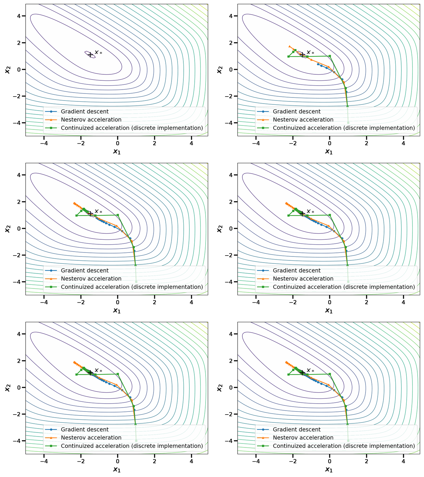
In this discrete implementation, the continuized acceleration performs similarly to Nesterov acceleration.
Conclusion
For practical purposes, Nesterov’s discrete acceleration wins. The iteration is elementary to implement and it enjoys a great performance. (There are exceptions in distributed optimization for which Nesterov acceleration would not enable asynchrony but the continuized acceleration does [1]).
For conceptual purposes, the continuous perspective on acceleration gives a crude intuition on the mechanism at play. However, there are also important aspects lost in the limit of small stepsizes, related to the choice of the discretization.
The continuized acceleration has two faces, continuous and discrete. As a discrete iteration, it is a randomized version of Nesterov’s original iteration. As a continuous process, it is more sophisticated that a simple ODE, as it involves random jumps. However, it gives a continuous-time perspective on acceleration without any conceptual loss.
References
[1] Mathieu Even, Raphaël Berthier, Francis Bach, Nicolas Flammarion, Hadrien Hendrikx, Pierre Gaillard, Laurent Massoulié, and Adrien Taylor. Continuized accelerations of deterministic and stochastic gradient descents, and of gossip algorithms. Advances in Neural Information Processing Systems 34 (2021): 28054-28066.
[2] Alexandre d’Aspremont, Damien Scieur, and Adrien Taylor. Acceleration methods. Foundations and Trends® in Optimization 5, no. 1-2 (2021): 1-245.
[3] Yurii Nesterov. Introductory lectures on convex optimization: A basic course. Vol. 87. Springer Science & Business Media, 2003.
[4] Weijie Su, Stephen Boyd, and Emmanuel Candes. A differential equation for modeling Nesterov’s accelerated gradient method: theory and insights. Advances in Neural Information Processing Systems 27 (2014).
[5] Bin Shi, Simon Du, Michael Jordan, and Weijie Su. Understanding the acceleration phenomenon via high-resolution differential equations. Mathematical Programming 195, no. 1 (2022): 79-148.
[6] Boris Polyak. Some methods of speeding up the convergence of iteration methods. USSR computational mathematics and mathematical physics, 4(5), pp.1-17 (1964).
[7] Lessard, Laurent, Benjamin Recht, and Andrew Packard. Analysis and design of optimization algorithms via integral quadratic constraints. SIAM Journal on Optimization 26, no. 1 (2016): 57-95.
[8] David Aldous and James Fill. Reversible Markov chains and random walks on graphs. Unpublished monograph (1995).
[9] Stephen Wright. Coordinate descent algorithms. Mathematical Programming 151, no. 1 (2015): 3-34.
[10] Hedy Attouch, Zaki Chbani, Juan Peypouquet, and Patrick Redont. Fast convergence of inertial dynamics and algorithms with asymptotic vanishing viscosity. Mathematical Programming 168, no. 1 (2018): 123-175.
[11] Sébastien Bubeck, Yin Tat Lee, and Mohit Singh. A geometric alternative to Nesterov’s accelerated gradient descent. arXiv preprint arXiv:1506.08187 (2015).
[12] Nicolas Flammarion and Francis Bach. From averaging to acceleration, there is only a step-size. In Conference on Learning Theory, pp. 658-695. PMLR (2015).
[13] Yossi Arjevani, Shai Shalev-Shwartz, and Ohad Shamir. On lower and upper bounds in smooth and strongly convex optimization. The Journal of Machine Learning Research 17, no. 1 (2016): 4303-4353.
[14] Donghwan Kim and Jeffrey Fessler. Optimized first-order methods for smooth convex minimization. Mathematical programming 159, no. 1 (2016): 81-107.
[15] Zeyuan Allen-Zhu and Lorenzo Orecchia. Linear coupling: An ultimate unification of gradient and mirror descent. In Proceedings of the 8th Innovations in Theoretical Computer Science ITCS’17 (2017).