Are all kernels cursed?

The word “kernel” appears in many areas of science (it is even worse in French with “noyau”); it can have different meanings depending on context (see here for a nice short historical review for mathematics).

Within machine learning and statistics, kernels are used in two related but different contexts, with different definitions and some kernels like the beloved and widely used Gaussian kernel being an example of both. This has been and still is a source of confusion that I would like to settle for good with this post! In particular, these two types of kernels have different properties regarding their resistance (or lack thereof) to the curse of dimensionality.

Throughout this post, for simplicity, I will assume that data live in \(\mathbb{R}^d\), noting that most concepts can be extended to any space (e.g., images, graphs, etc.): this is the beauty of the (positive-definite) kernel trick but this is for another post.

I will consider a kernel function \(k\), which is a real-valued function defined on \(\mathbb{R}^d \times \mathbb{R}^d\). I will always assume that the kernel \(k\) is symmetric, that is, \(k(x,y) = k(y,x)\) for any \(x,y \in \mathbb{R}^d\).

An important object of study will be the kernel matrix \(K \in \mathbb{R}^{n \times n}\) obtained from \(n\) observations \(x_1,\dots,x_n \in\mathbb{R}^d\), which is defined through $$K_{ij} = k(x_i,x_j).$$ Given the symmetry assumption on \(k\), it will be a symmetric matrix (hence with real eigenvalues).

I will now present the two types of kernels, (1) non-negative kernels and (2) positive-definite kernels. For kernels of the form \(k(x,y) = q(x-y)\) for a function \(q: \mathbb{R}^d \to\mathbb{R}\), the two definitions will correspond to (1) \( q \) has non-negative values, and (2) the Fourier transform of \(q\) has non-negative values. This leads to different types of algorithms that I now present.

I. Non-negative kernels

Definition (non-negative kernels). A kernel \(k: \mathbb{R}^d \times \mathbb{R}^d \to \mathbb{R}\) is non-negative, if $$\forall x,y \in \mathbb{R}^d, \ k(x,y) \geq 0.$$

An equivalent definition is that all kernel matrices have non-negative elements. The explicit terminology pointwise non-negativity is sometimes used.

The most classical example is the Gaussian kernel, defined as $$k(x,y) = \exp\Big( -\frac{1}{2 \sigma^2} \| x – y\|_2^2\Big),$$ where \(\| z\|_2^2 = \sum_{i=1}^d z_i^2\) is the squared \(\ell_2\)-norm (I have not added any normalizing constant because most algorithms ignore it). Other examples are shown below for \(d=1\).

There are many more choices (see here), but the functions below all also have a non-negative Fourier transform, which will make them also a member of the other class of kernels (see the second part of the post).

Kernel smoothing (a.k.a. Nadaraya-Watson estimator)

This is a version of kernel density estimation for supervised problems, which for simplicity I will describe with real-valued outputs (it can directly be extended to any generalized linear model to tackle other types of outputs). Given \(n\) observations \((x_i,y_i) \in \mathbb{R}^d \times \mathbb{R}\), \(i=1,\dots,n\), the goal of kernel smoothing is to estimate a function \(\hat{f}: \mathbb{R}^d \to \mathbb{R}\) that can predict \(y\) from \(x\). It is defined at any test point \({x} \in \mathbb{R^d}\): $$\hat{f}(x) = \frac{\sum_{i=1}^n k(x,x_i) y_i}{\sum_{i=1}^n k(x,x_i)}.$$

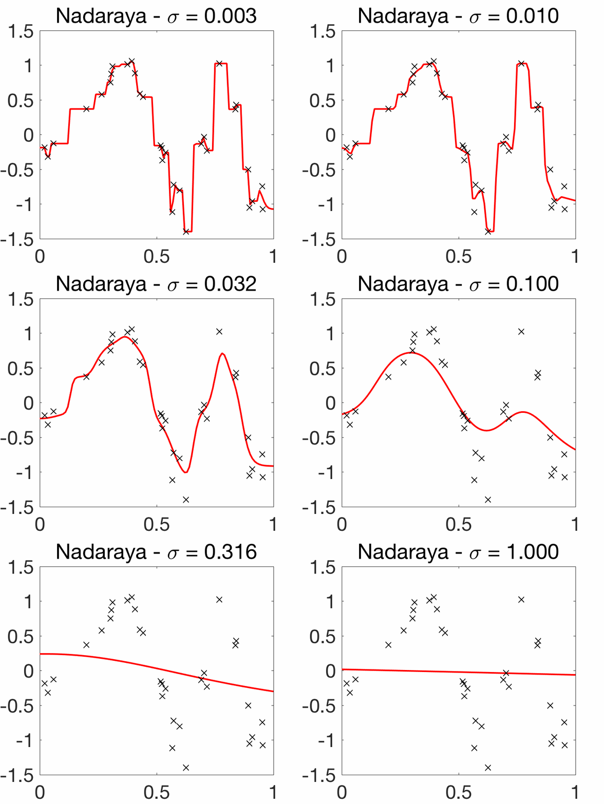
See an illustrative example below in one dimension for the Gaussian kernel. The non-negativity of the kernel is important to make sure the denominator above is positive.

Algorithms. In terms of computational complexity, computing \(\hat{f}(x)\) for a single \(x\) takes naively time \(O(n)\) to go through the \(n\) data points, but efficient indexing techniques such as k-d trees can be used to reduce this cost when \(d\) is not too large. The vector of prediction \(\hat{y}\) for the \(n\) observations, can be obtained as $$ \hat{y} = {\rm Diag}(K 1_n)^{-1} K y .$$ The complexity is \(O(n^2)\) but can also be made linear in \(n\) (in particular when the kernel matrix is in addition positive semi-definite, i.e., when the kernel is both non-negative and positive-definite).

It is important to note that the only free parameter is the bandwidth \(\sigma\), while there will be an extra regularization parameter for positive definite kernels.

Choice of bandwidth. As illustrated below, for kernels of the form \(k(x,y) = q\big( \frac{x-y}{\sigma} \big)\), like the Gaussian kernel, the choice of the bandwidth parameter \(\sigma\) is crucial.

Note here that when \(\sigma\) tends to zero, then the estimated function \(\hat{f}\) interpolates the data (but without any wild behavior between input observations), while when \(\sigma\) grows, the function \(\hat{f}\) tends to a constant. We now consider only these translation-invariant kernels.

Statistical properties. Kernel smoothing is a simple instance of a non-parametric estimation procedure, that can in principle adapt to any underlying function \(f\) that generated the outputs (after additive noise is added, so that the observations are \(y_i = f(x_i) + \varepsilon_i\), with \(\varepsilon_i\) being zero-mean). This estimator is commonly used in low dimensions (e.g., \(d\) less than \(10\) or \(20\)). In higher dimensions however, it suffers from the curse of dimensionality common to most methods based on non-negative kernels.

Consistency and curse of dimensionality. Kernel regression is one instance of local averaging techniques such as k-nearest-neighbors, where for any test point \(x\), the outputs \(y_i\) corresponding to inputs \(x_i\) which are closer to \(x\) are given higher weights. For simplicity, I will only consider the kernel \(k(x,y) = 1_{\| x – y\|_\infty \leq \sigma}\) where \(\| z\|_\infty = \max\{ |z_1|,\dots,|z_d|\}\) is the \(\ell_\infty\)-norm of \(z\). The discussion below extends with more technicalities to all translation-invariant kernels.

In order to obtain a consistent estimator \(\hat{f}\) that converges to the true underlying function \(f\) when \(n\) tends to infinity, the bandwidth \(\sigma\) should depend on \(n\) (and hence denoted \(\sigma_n\)), with two potentially conflicting goals:

• Vanishing bias: The bandwidth \(\sigma_n\) should be small enough so that the underlying function \(f\) does not vary much in a ball of radius \(\sigma_n\) around \(x\). When \(f\) is assumed Lipschitz-continuous, the deviation is proportional to \(\sigma_n\). Therefore, the error in estimating \(f\) is proportional to \(\sigma_n\) and we thus need $$ \sigma_n \to 0.$$
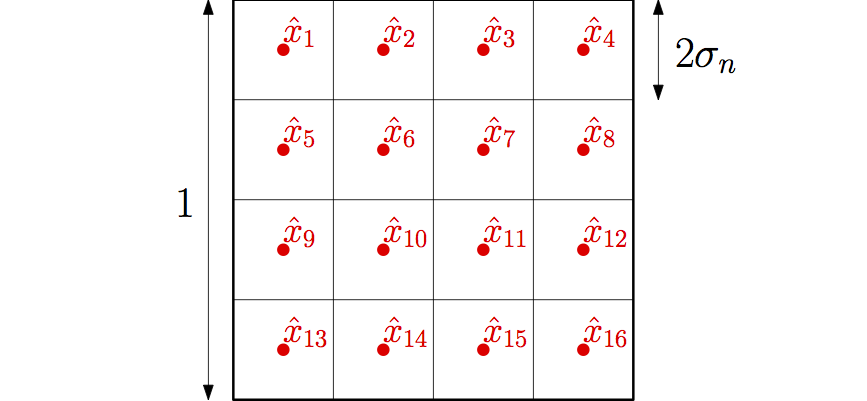
• Vanishing variance: Since the observations \(y_i = f(x_i) + \varepsilon_i\) are noisy, around some test point \(\hat{x}\), we need to average sufficiently many of them so that the noise is averaged out, that is, for any test point \(\hat{x}\), the number of observations that are in a ball of radius \(\sigma_n\) should tend to infinity with \(n\). With a simple covering argument, this requires (at least) $$ n \sigma_n^d \to +\infty.$$ This illustrated below for the specific kernel I chose, which is based on the \(\ell_\infty\)-norm.

Therefore, in order to obtain a consistent estimator, the bandwidth of translation-invariant kernels has to go to zero slowly enough, slower than \(n^{-1/d}\), and the final estimation error is converging to zero, but slower than \(n^{-1/d}\). This is the usual curse of dimensionality: in order to obtain a certain error \(\epsilon\), the number of observations has to grow at least as \(\epsilon^{-d}\), and thus exponentially in dimension. When the underlying function has weak smoothness properties (here just Lipschitz-continuous), such a dependence in \(d\) is provably unavoidable in general [1, 2].

Resistance to the curse of dimensionality. If the true function \(f\) happens to be more regular (i.e., with bounded higher order derivatives), kernel smoothing cannot adapt to it, that is, the rates of convergence still have the bad dependence on \(d\), while other techniques can have an improved dependence, such as positive-definite kernel methods below, or improved local averaging techniques based on local polynomials [1, 2].

Note that since the curse of dimensionality comes primarily from a covering argument of the input space, if the distribution of inputs is supported on a low-dimensional manifold, the dependence in \(d\) can be replaced by the same dependence, but now in the dimension of the manifold (see, e.g., [7]).

Kernel smoothing is one particular instance of methods based on negative-kernels. kernel density estimation is also commonly used. Spectral methods for clustering and non-linear dimensionality reduction, and Laplacian-based semi-supervised learning [8], also use non-negative kernels, with similar conditions on the bandwidth \(\sigma\) (see [3]) and similar curses of dimensionality.

I now turn to the other type of kernels.

II. Positive-definite kernels

Definition (positive-definite kernels). A kernel \(k: \mathbb{R}^d \times \mathbb{R}^d \to \mathbb{R}\) is positive-definite, if for any finite set of elements \(x_i,\dots,x_n\) in \(\mathbb{R}^d\), the kernel matrix is positive-semidefinite (that is, all its eigenvalues are non-negative).

The classical examples are:

• Polynomial kernels: \(k(x,y) = (x^\top y)^r\) for \(r\) a positive integer.
• Translation-invariant kernels: they are of the form \(k(x,y) = q(x-y)\) for a function \(q: \mathbb{R}^d \to \mathbb{R}\) with a (pointwise) non-negative Fourier transform, which is equal to\(\displaystyle \hat{q}(\omega) = \int_{\mathbb{R}^d} \! \! q(x) e^{-i \omega^\top x} dx\), and assumed to exist. For these, we see a clear distinction between non-negative kernels of that form, for which \(q\) (and not \(\hat{q}\)) has to have non-negative elements (note that all examples given at the beginning of the post are both, and that there are two hidden Fourier transform pairs).
• Kernels on structured objects: when the observations are not vectors in \(\mathbb{R}^d\), such as graphs, trees, measures, on in fact any objects, specific kernels can be designed with nice properties and many applications, see, e.g., [4].

Kernel trick and representer theorem

The key consequence of positive-definiteness (with surprisingly no other assumptions needed regarding \(k\)) is the existence of an (essentially unique) Hilbert space \(\mathcal{F}\), called the feature space, and a function \(\Phi: \mathbb{R}^d \to \mathcal{F}\), called the feature map, such that $$\forall x,y \in \mathbb{R}^d, \ k(x,y) = \langle \Phi(x), \Phi(y) \rangle_\mathcal{F}.$$ This is non-trivial to show and due to Aronszajn and Moore in the 1950s.

From a positive-definite kernel, it is to common to define the space of functions \(f\) which are linear in the feature vector \(\Phi\), that is, of the form \(f(x) = \langle w, \Phi(x) \rangle_{\mathcal{F}}\), for a certain \(w \in \mathcal{F}\). When minimizing an empirical risk on \(n\) observations \(x_1,\dots,x_n \in \mathbb{R}^d\), regularized by the norm \(\| w\|_\mathcal{F}\), the celebrated representer theorem (which is a direct consequence of Pythagoras’ theorem) states that \(w\) is of the form \(w = \sum_{j=1}^n \alpha_j \Phi(x_j)\), and thus \(f\) is of the form $$f(x) = \sum_{j=1}^n \alpha_j \langle \Phi(x), \Phi(x_j) \rangle_\mathcal{F} = \sum_{j=1}^n \alpha_j k(x,x_j),$$ for a certain vector \(\alpha \in \mathbb{R}^n\).

Regularization through positive-definite kernels

Given the function \(f\) defined as \(f(x) = \langle w, \Phi(x) \rangle_{\mathcal{F}}\), the regularizer \(\| w\|_\mathcal{H}\) defines a regularization on the prediction function \(f\). This is a key property of positive-definite kernels: they lead to an explicit regularization \(\Omega(f)^2\) on the prediction function (this in fact defines a Hilbert space of functions, which is often referred to as the reproducing kernel Hilbert space).

For the translation-invariant kernels \(k(x,y) = q(x-y)\), it happens to be equal to (see [4]) $$ \Omega(f)^2 =\frac{1}{(2\pi)^d} \int_{\mathbb{R}^d} \!\! \frac{|\hat{f}(\omega)|^2 }{\hat{q}(\omega)} d\omega,$$ where \(\hat{f}\) and \(\hat{q}\) are the Fourier transforms of \(f\) and \(q\). For example, for \(d=1\) and the exponential kernel \(q(x-y) = \exp(-|x-y|/\sigma)\), we have \(\hat{q}(\omega) = 2 \sigma / ( 1 + \sigma^2 \omega^2)\), and \(\displaystyle \Omega(f)^2= \frac{1}{2\sigma} \int_{\mathbb{R}} \! |f(x)|^2 dx +\frac{ \sigma}{2} \int_{\mathbb{R}}\! |f'(x)|^2 dx \), which is a squared Sobolev norm (this extends to higher dimensions as well).

In addition, for the Gaussian kernel \(q(x-y) = \exp \big(-(x-y)^2/(2\sigma^2) \big)\), we have \(\hat{q}(\omega) = \sigma \sqrt{2\pi} \exp( – \sigma^2 \omega^2 / 2)\), and \(\displaystyle \Omega(f)^2 = \frac{1}{\sigma \sqrt{2\pi}}\sum_{k=0}^\infty \frac{\sigma^{2k}}{2^k k!}\! \int_{\mathbb{R}} \!|f^{(k)}(x)|^2 dx\), and all derivatives are penalized (also, this extends in higher dimensions).

Finally, some versions of splines can be obtained from positive-definite kernels (and kernel ridge regression below exactly leads to smoothing splines).

Kernel ridge regression

As a consequence of the representer theorem above, when using the square loss, and for a vector of outputs / responses \(y \in \mathbb{R}^n\), when minimizing $$ \frac{1}{n} \sum_{i=1}^n \big( y_i – \langle w, \Phi(x_i) \rangle_{\mathcal{F}} \big)^2 + \lambda \| w\|_\mathcal{F}^2,$$ the \(i\)-th prediction \( \langle w, \Phi(x_i) \rangle_{\mathcal{F}}\) is equal to \(\sum_{j=1}^n \alpha_j \langle \Phi(x_j),\Phi(x_i)\rangle_{\mathcal{F}}=(K\alpha)_i\) and \(\| w\|_\mathcal{F}^2\) is equal to \(\sum_{i,j=1}^n \alpha_i \alpha_j K_{ij} = \alpha^\top K \alpha\). This leads to the equivalent problem of minimizing $$ \frac{1}{n} \| y – K \alpha \|_2^2 + \lambda \alpha^\top K \alpha,$$ with a solution \(\alpha = ( K + n\lambda I)^{-1} y \in \mathbb{R}^n\), and prediction vector \(\hat{y} = K ( K+ n\lambda I)^{-1} y \in \mathbb{R}^n\).

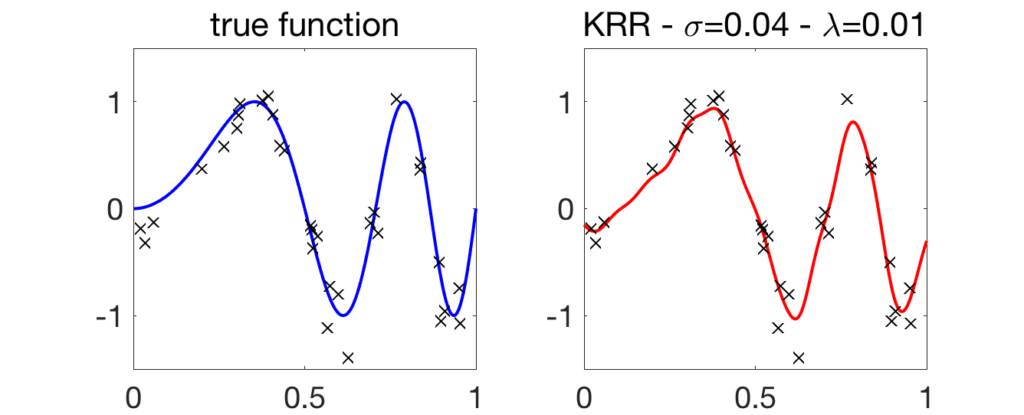
See an illustration below for the Gaussian kernel.

Running-time complexity. Implemented naively in a few lines of code, the complexity will be \(O(n^2)\) for computing the kernel matrix \(K\) and \(O(n^3)\) for solving the linear system to obtain \(\alpha\). This can be greatly reduced using low-rank approximations (a.k.a. Nyström’s method) or random features [5]. More on these in future posts.

Do we really need positive-definiteness? In the objective function above, the only place where positive-definiteness seems needed is for the the regularization term \(\alpha^\top K \alpha\) to be convex, which automatically leads to a well-behaved optimization problem. We could do the same by replacing it by \(\| \alpha\|_2^2\) and no need for \(K\) to be positive-semidefinite. While this is implementable, it lacks a clear interpretation in terms of regularization of the prediction function and some of the techniques designed to avoid a running time complexity of \(O(n^2)\) cannot be used.

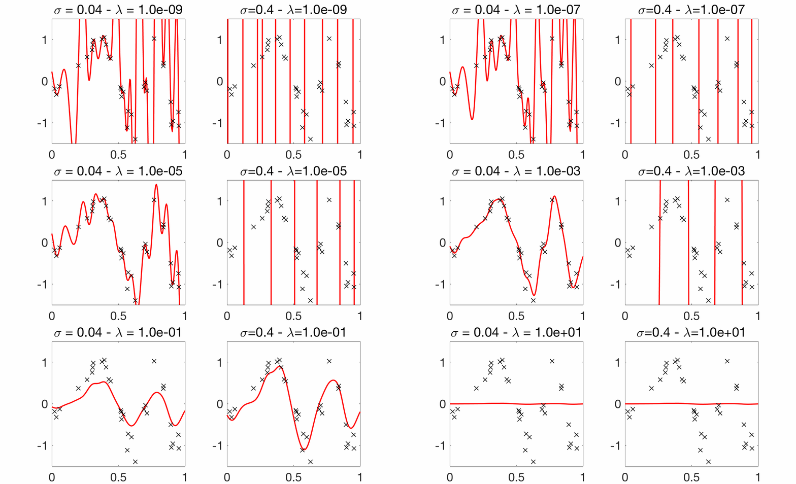
Choice of bandwidth. Compared to the Nadaraya-Watson estimator, for translation-invariant kernels, there are two parameters, the kernel bandwidth \(\sigma\) and the regularization parameter \(\lambda\). Below, we vary \(\lambda\) for two fixed values of \(\sigma\). A few points to note:

• Strong overfitting for small \(\lambda\): compared to Nadaraya-Watson, which was interpolating nicely for small \(\sigma\), kernel ridge regression overfits a lot for small \(\lambda\), with a wild behavior between observed inputs.
• Robustness to larger \(\sigma\): with a proper regularization parameter \(\lambda\), larger values of \(\sigma\) can still lead to good predictions (as opposed to Nadaraya-Watson estimation). Another illustration of the robustness to larger \(\sigma\) is the possibility of having consistent estimation without a vanishing bandwidth \(\sigma\) (see below).

Consistency and curse of dimensionality

Positive-definite kernel methods are also non-parametric estimation procedures. They can adapt to any underlying function, if the kernel is universal. For translation-invariant kernels, a sufficient condition is a strictly positive Fourier transform (which is typically true for all bandwidths).

In most analyses, the bandwidth \(\sigma\) is fixed, and the regularization parameter \(\lambda\) goes to zero with \(n\) (a notable exception is the nice paper from the Vert brothers [6]). With the proper decay of \(\lambda\), as \(n\) grows, we obtain a consistent estimator.

When only assuming Lipschitz-continuity of the true underlying function, the rate of convergence also has a bad behavior in dimension \(d\), typically of the form \(O(n^{-1/d})\) (any way, such dependence is provably unavoidable, this is the usual curse of dimensionality for regression in high dimension).

Adaptivity to smooth functions. A key benefit of using positive-definite kernels is that if the underlying function is smoother than simply Lipschitz-continuous, then the convergence rates do improve with a proper choice of \(\lambda\). In the most favorable situation where the true regression function \(f\) belongs to the space of functions defined by the kernel, then the convergent rate is less than \(O(n^{-1/4})\). This may however require functions which are too smooth (in particular for the Gaussian kernel, these functions are infinitely differentiable).

However, kernel methods also lead to consistent estimation beyond this favorable situation, and such methods are adaptive to all functions which are in between Lipschitz-continuous functions (essentially bounded first order derivatives) and these potentially very smooth functions. For example, for the Gaussian kernel, as soon as it is \(s\)-times differentiable with bounded \(s\)-th order derivative, with \(s>d/2\), then the convergence rate does not exhibit any more a dependence in \(d\) in the power of \(n\), i.e., the convergence rate is also less than \(O(n^{-1/4})\). If \(s\) is smaller than \(d/2\), then the convergence rate is in between \(O(n^{-1/4})\) and \(O(n^{-1/d})\), essentially of the form \(O(n^{-2s/d})\) or \(O(n^{-s/d})\) (for precise details, see [1, 2]).

This adaptivity requires the proper regularization parameter \(\lambda\). For the Gaussian kernel, as outlined in [9], it may need to be very small (e.g., exponentially decaying with \(n\)), leading to optimization problems which are strongly ill-conditioned. More on this in a future post.

Conclusion

Are all kernels cursed? In this post, I have tried to highlight the difference between the two types of kernels, (1) the (pointwise) non-negative ones, which lead to local averaging techniques that cannot avoid the curse of dimensionality, even in favorable situations, and (2) the positive-definite ones, which exhibit some form of adaptivity.

If you went that far into the post, you are probably a kernel enthusiast, but if you are not and wondering why you should care about kernels in the neural network age, a few final thoughts:

• What are the adaptivity properties of neural networks? They are indeed superior; for example, with a single hidden layer, neural networks are adaptive to linear structures, such as dependence on a subset of variables, while kernels with similar architectures are not [10]. However, neural networks do not lead (yet) to precise guarantees on the solvability of the corresponding optimization problems.
• Can we learn with positive-definite kernels with lots of data? Yes! With proper tools such as random features [5] or column sampling, and with the proper and very nice pre-conditioning of [11], kernels can be used with ten millions of observations or more.
• Can we apply kernels to computer vision? Yes! See the nice blog post of Julien Mairal.
• Kernel methods as “theoretically tractable” high-dimensional models. In recent years, new ideas have emerged from training overparameterized neural networks, with (1) global convergence guarantees [12, 13], some of them related to kernel methods [14, 15], and (2) a new phenomenon called “double descent” [16], which has a nice theoretical explanation / illustration with kernel methods. Again topics for future (shorter) posts.

References

[1] László Györfi, Michael Kohler, Adam Krzyzak, Harro Walk. A distribution-free theory of nonparametric regression. Springer, 2006.
[2] Alexandre B. Tsybakov. Introduction to Nonparametric Estimation. Springer, 2009.
[3] Matthias Hein, Jean-Yves Audibert, Ulrike von Luxburg, Graph Laplacians and their convergence on random neighborhood graphs. Journal of Machine Learning Research, 8(Jun):1325-1368, 2007.
[4] Nello Cristianini and John Shawe-Taylor. Kernel Methods for Pattern Analysis. Cambridge University Press, 2004.
[5] Ali Rahimi, Benjamin Recht. Random Features for Large-Scale Kernel Machines. Advances in Neural Information Processing Systems (NIPS), 2007.
[6] Régis Vert, Jean-Philippe Vert. Consistency and Convergence Rates of One-Class SVMs and Related Algorithms. Journal of Machine Learning Research, 7(May):817-854, 2006.
[7] Peter J. Bickel, and Bo Li. Local polynomial regression on unknown manifolds. Complex datasets and inverse problems. Institute of Mathematical Statistics, 177-186, 2007.
[8] Xiaojin Zhu, Zoubin Ghahramani, John D. Lafferty. Semi-supervised learning using gaussian fields and harmonic functions. Proceedings of the International conference on Machine learning (ICML). 2003.
[9] Francis Bach. Sharp analysis of low-rank kernel matrix approximations. Proceedings of the International Conference on Learning Theory (COLT), 2003.
[10] Francis Bach. Breaking the Curse of Dimensionality with Convex Neural Networks. Journal of Machine Learning Research, 18(19):1-53, 2017.
[11] Alessandro Rudi, Luigi Carratino, Lorenzo Rosasco. FALKON: An Optimal Large Scale Kernel Method. Advances in Neural Information Processing Systems (NIPS), 2017.
[12] Lénaïc Chizat, Francis Bach. On the Global Convergence of Gradient Descent for Over-parameterized Models using Optimal Transport. Advances in Neural Information Processing Systems (NeurIPS), 2018.
[13] Song Mei, Andrea Montanari, and Phan-Minh Nguyen. A mean field view of the landscape of two-layer neural networks. Proceedings of the National Academy of Sciences (PNAS), 115(33):E7665–E7671, 2018.
[14] Arthur Jacot, Franck Gabriel, Clément Hongler. Neural tangent kernel: Convergence and generalization in neural networks. Advances in neural information processing systems (NeurIPS), 2018.
[15] Lénaïc Chizat, Edouard Oyallon, Francis Bach. On Lazy Training in Supervised Differentiable Programming. Arxiv-1812.07956, 2018.
[16] Mikhail Belkin, Daniel Hsu, Siyuan Ma, Soumik Mandal. Reconciling modern machine learning practice and the bias-variance trade-off. Proceedings of the National Academy of Sciences (PNAS), 116 (32), 2019.