Gradient descent for wide two-layer neural networks – II: Generalization and implicit bias

In this blog post, we continue our investigation of gradient flows for wide two-layer “relu” neural networks. In the previous post, Francis explained that under suitable assumptions these dynamics converge to global minimizers of the training objective. Today, we build on this to understand qualitative aspects of the predictor learnt by such neural networks. The content is mostly based on our recent joint work [1].

1. Generalization with weight decay regularization

Let us start our journey with the comfortable case where the training objective includes an explicit weight decay regularization (i.e. \(\ell_2\)-regularization on the parameters). Using the notations of the previous post, this consists in the following objective function on the space of probability measures on \(\mathbb{R}^{d+1}\): $$ \underbrace{R\Big(\int_{\mathbb{R}^{d+1}} \Phi(w)d\mu(w)\Big)}_{\text{Data fitting term}} + \underbrace{\frac{\lambda}{2} \int_{\mathbb{R}^{d+1}} \Vert w \Vert^2_2d\mu(w)}_{\text{Regularization}} \tag{1}$$ where \(R\) is the loss and \(\lambda>0\) is the regularization strength. Remember that a neural network of finite width with \(m\) neurons is recovered with an empirical measure \(\mu = \frac1m \sum_{j=1}^m\delta_{w_j}\), in which case this regularization is proportional to the sum of the squares of all the parameters \(\frac{\lambda}{2m}\sum_{j=1}^m \Vert w_j\Vert^2_2\).

Variation norm. In the previous post, we have seen that the Wasserstein gradient flow of this objective function — an idealization of the gradient descent training dynamics in the large width limit — converges to a global minimizer \(\mu^*\) when initialized properly. An example of an admissible initialization is the hidden weights \(b_j\) distributed according to the uniform distribution \(\tau\) on the unit sphere \(\mathbb{S}^{d-1}\subset \mathbb{R}^d\) and the output weights \(a_j\) uniform in \(\{-1,1\}\). What does this minimizer look like in predictor space when the objective function is as in Eq. (1) ?

To answer this question, we define for a predictor \(h:\mathbb{R}^d\to \mathbb{R}\), the quantity $$ \Vert h \Vert_{\mathcal{F}_1} := \min_{\mu \in \mathcal{P}(\mathbb{R}^{d+1})} \frac{1}{2} \int_{\mathbb{R}^{d+1}} \Vert w\Vert^2_2 d\mu(w) \quad \text{s.t.}\quad h = \int_{\mathbb{R}^{d+1}} \Phi(w)d\mu(w).\tag{2} $$ As the notation suggests, \(\Vert \cdot \Vert_{\mathcal{F}_1}\) is a norm in the space of predictors. It is known as the variation norm [2, 3]. We call \(\mathcal{F}_1\) the space of functions with finite norm, which is a Banach space. By construction, the learnt predictor \(h^* = \int \Phi(w)d\mu^*(w)\) is a minimizer of the \(\mathcal{F}_1\)-regularized regression: $$ \min_{h:\mathbb{R}^d\to \mathbb{R}} R(h) + \lambda \Vert h \Vert_{\mathcal{F}_1} \tag{3}.$$ This \(\mathcal{F}_1\)-norm regularization shares similarity with \(\ell_1\) regularization [4]. To see this, observe that the “magnitude” \(\vert a\vert \Vert b\Vert_2\) of a relu function \(x\mapsto a(b^\top x)_+\) with parameter \(w=(a,b)\) equals \(\Vert w\Vert^2_2/2\) if \(\vert a\vert = \Vert b\Vert_2\) and is smaller otherwise. Thus parameterizing the relus by their direction \(\theta = b/\Vert b\Vert_2\) and optimizing over their signed magnitude \(r(\theta) = a\Vert b\Vert_2\) we have $$ \Vert h \Vert_{\mathcal{F}_1} = \inf_{r:\mathbb{S}^{d-1}\to \mathbb{R}} \int_{\mathbb{S}^{d-1}} \vert r(\theta)\vert d\tau(\theta) \quad \text{s.t.}\quad h(x) = \int _{\mathbb{S}^{d-1}} r(\theta) (\theta^\top x)_+ d\tau(\theta).\tag{4}$$

Conjugate RKHS norm. The regression in the space \(\mathcal{F}_1\) is best understood when compared with the regression obtained by only training the output weights. We consider the same training dynamics with weight decay except that we fix the hidden weights to their initial value, where they are distributed according to the uniform distribution \(\tau\) on the sphere. In that case, the Wasserstein gradient flow also converges to the solution of a regularized regression as in Eq. (3) — this is in fact a convex problem — but the regularizing norm is different and now defined as $$ \Vert h \Vert_{\mathcal{F}_2}^2 := \min_{r:\mathbb{S}^{d-1}\to \mathbb{R}} \int_{\mathbb{S}^{d-1}} \vert r(\theta)\vert^2 d\tau(\theta) \quad \text{s.t.}\quad h(x) = \int _{\mathbb{S}^{d-1}} r(\theta) (\theta^\top x)_+ d\tau(\theta).$$ We call \(\mathcal{F}_2\) the set of functions with finite norm. It can be shown to be a Reproducing Kernel Hilbert Space (RKHS), with kernel $$ K(x,x’) = \int_{\mathbb{S}^{d-1}} (\theta^\top x)_+ (\theta^\top x’)_+ d\tau(\theta),$$ which has a closed form expression [5]. In this context, taking a finite width neural network corresponds to a random feature approximation of the kernel [6, 7].

Let us informally compare the properties of these spaces \(\mathcal{F}_1\) and \(\mathcal{F}_2\) (see [2] for details):

• Approximation power. In high dimension, only very smooth functions have small \(\mathcal{F}_2\)-norm (in rough terms, the \(\lceil (d+3)/2\rceil\) first derivatives should be small). In contrast, there exists non-smooth functions with small \(\mathcal{F}_1\)-norm, an example being the relu function \(x\mapsto (\theta^\top x)_+\). Remarkably, if we define \(f(x)=g(Ux)\) where \(U\) is an orthogonal projection then \(\Vert f\Vert_{\mathcal{F}_1} \leq \Vert g\Vert_{\mathcal{F}_2}\). This shows in particular that \(\mathcal{F}_1\) contains \(\mathcal{F}_2\) and that \(\mathcal{F}_1\) is adaptive to lower dimensional structures.
• Statistical complexity. It could be feared that the good approximation properties of \(\mathcal{F}_1\) come at the price of being “too large” as a hypothesis space, making it difficult to estimate a predictor in \(\mathcal{F}_1\) from few samples. But, as measured by their Rademacher complexities, the unit ball of \(\mathcal{F}_1\) is only \(O(\sqrt{d})\) larger than that of \(\mathcal{F}_2\). By going from \(\mathcal{F}_2\) to \(\mathcal{F}_1\), we thus add some nicely structured predictors to our hypothesis space, but not too much garbage that could fit unstructured noise.
• Generalization guarantees. By combining the two previous points, it is possible to prove that supervised learning in \(\mathcal{F}_1\) breaks the curse of dimensionality when the output depends on a lower dimensional projection of the input: the required number of training samples only depends mildly on the dimension \(d\).
• Optimization guarantees. However \(\mathcal{F}_1\) has a strong drawback : there is no known algorithm that solves the problem of Eq. (3) in polynomial time. On practical problems, gradient descent seems to behave well, but in general only qualitative results such as presented in the previous post are known. In contrast, various provably efficient algorithms can solve regression in \(\mathcal{F}_2\), which is a classical kernel ridge regression problem [Chap. 14.4.3, 8].

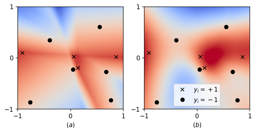
In the plot below, we compare the predictor learnt by gradient descent for a 2-D regression with the square loss and weight decay, after training (a) both layers — which is regression in \(\mathcal{F}_1\) — or (b) just the output layer — which is regression in \(\mathcal{F}_2\). This already illustrates some distinctive features of both spaces, although the differences become more stringent in higher dimensions. In particular, observe that in (a) the predictor is the combination of few relu functions, which illustrates the sparsifying effect of the \(L^1\)-norm in Eq. (4). To simplify notations, we do not include a bias/intercept in the formulas but our numerical experiments include it, so in this plot the input is of the form \(x=(x_1,x_2,1)\) and \(d=3\).

The qualitative picture is quite clear so far, but something is a bit unsettling: weight decay is often not needed to obtain a good performance in practice. Our line of reasoning however completely falls apart without such a regularization: if the objective function depends on the predictor only via its values on the training set, being a minimizer does not guarantee anything about generalization outside of the training set (remember that wide relu neural networks are universal approximators). Why does it still work in the unregularized case? There must be something in the algorithm…

2. Implicit bias: linear classification

This something is called the implicit bias : when there are several minimizers, the optimization algorithm makes a specific choice. In the unregularized case, the “quality” of this choice is a crucial property of an algorithm; much more crucial than, say, its convergence speed on the training objective. To gradually build our intuition of the implicit bias of gradient flows, let us put neural networks aside for a moment and consider, following Soudry, Hoffer, Nacson, Gunasekar and Srebro [9], a linear classification task.

Gradient flow of the smooth-margin. Let \((x_i,y_i)_{i=1}^n\) be a training set of \(n\) pairs of inputs \(x_i\in \mathbb{R}^d\) and outputs \(y_i\in \{-1,1\}\) and let us choose the exponential loss. The analysis that follows also apply to the logistic loss (which is the same as the cross-entropy loss after a sigmoid non-linearity) because only the “tail” of the loss matters, but it is more straightforward with the exponential loss. In order to give a natural “scale” to the problem, we renormalize the empirical risk by taking minus its logarithm and consider the concave objective $$ F_\beta(a) = -\frac{1}{\beta}\log\Big( \frac1n \sum_{i=1}^n \exp(-\beta y_i \ x_i^\top a) \Big).\tag{5}$$

Here \(\beta>0\) is a parameter that will be useful in a moment. For now, we take \(\beta=1\) and we note \(F(a)=F_1(a)\). In this context, the margin of a vector \(a\in \mathbb{R}^d\) is the quantity \(\min_{i} y_i\ x_i^\top a\) which quantifies how far this linear predictor is from making a wrong prediction on the training set.

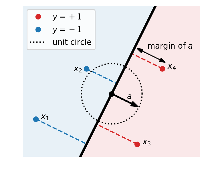
Obtained via simple manipulations, the inequalities $$ \min_i y_i\ x_i^\top a \leq F_\beta(a) \leq \min_i y_i\ x_i^\top a +\frac{\log(n)}{\beta}, \tag{6}$$ suggest to call \(F_\beta\) the smooth-margin because, well, it is smooth and converges to the margin \(F_\infty(a) := \min_i y_i x_i^\top a\) as \(\beta\to \infty\). Let us look at the gradient flow in the ascent direction that maximizes the smooth-margin: $$ a'(t) = \nabla F(a(t))$$ initialized with \(a(0)=0\) (here the initialization does not matter so much). The path followed by this gradient flow is exactly the same as the gradient flow on the empirical risk: taking the logarithm only changes the time parameterization or, in practice, the step-size.

Convergence to the max-margin. Assume that the data set is linearly separable, which means that the \(\ell_2\)-max-margin $$ \gamma := \max_{\Vert a\Vert_2 \leq 1} \min_i y_i x_i^\top a$$ is positive. In this case \(F\) is unbounded (indeed \(\lim_{\alpha \to \infty} F(\alpha a) =\infty\) whenever \(a\) has a positive margin) and thus \(a(t)\) diverges. This is not an issue as such, since for classification, only the sign of the prediction matters. This just means that the relevant question is not “where does \(a(t)\) converge?” but rather “towards which direction does it diverge?”. In other words, we are interested in the limit of \(\bar a(t):= a(t)/\Vert a(t)\Vert_2\) (in convex analysis, this is called the cosmic limit of \(a(t)\) [Chap. 3, 10], isn’t it beautiful ?).

The argument that follows is adapted from [11, 12] and can be traced back to [13] for coordinate ascent. It can be shown by looking at the structure of the gradient (see the end of the blog post) that \(\Vert \nabla F(a)\Vert_2\geq \gamma\) for all \(a\in \mathbb{R}^d\). By the inequality of Eq. (6) and the gradient flow property \(\frac{d}{dt}F(a(t))=\Vert \nabla F(a(t))\Vert_2^2\), it follows $$\begin{aligned}\min_i y_i x_i^\top a(t) \geq F(a(t)) \ – \log(n) \geq \gamma \int_0^t \Vert \nabla F(a(s))\Vert_2ds -\log (n).\end{aligned}$$ For \(t> \log(n)/\gamma^2\), this lower bound is positive. We can then divide the left-hand side by \(\Vert a(t)\Vert_2\) and the right-hand side by the larger quantity \(\int_0^t \Vert\nabla F(a(s))\Vert_2ds\), and we get $$\min_i y_i x_i^\top \bar a(t) \geq \gamma -\frac{\log(n)}{\int_0^t \Vert\nabla F(a(s))\Vert_2ds} \geq \gamma -\frac{\log(n)}{\gamma t}.$$ This shows that the margin of \(\bar a(t) := a(t)/\Vert a(t)\Vert_2\) converges to the \(\ell_2\)-max-margin at a rate \(\log(n)/\gamma t\). That’s it, the implicit bias of this gradient flow is exposed!

Stability to step-size choice. To translate this argument to discrete time, we need decreasing step-sizes of order \(1/\sqrt{t}\) which deteriorates the convergence rate to \(\tilde O(1/\sqrt{t})\), see [11, 12]. In [1], we proposed a different proof strategy (based on an online optimization interpretation of \(\bar a(t)\), as below) which recovers the same convergence rate \(O(1/\sqrt{t})\) with exponentially larger step-sizes. This suggests that these diverging trajectories are extremely robust to the choice of step-size.

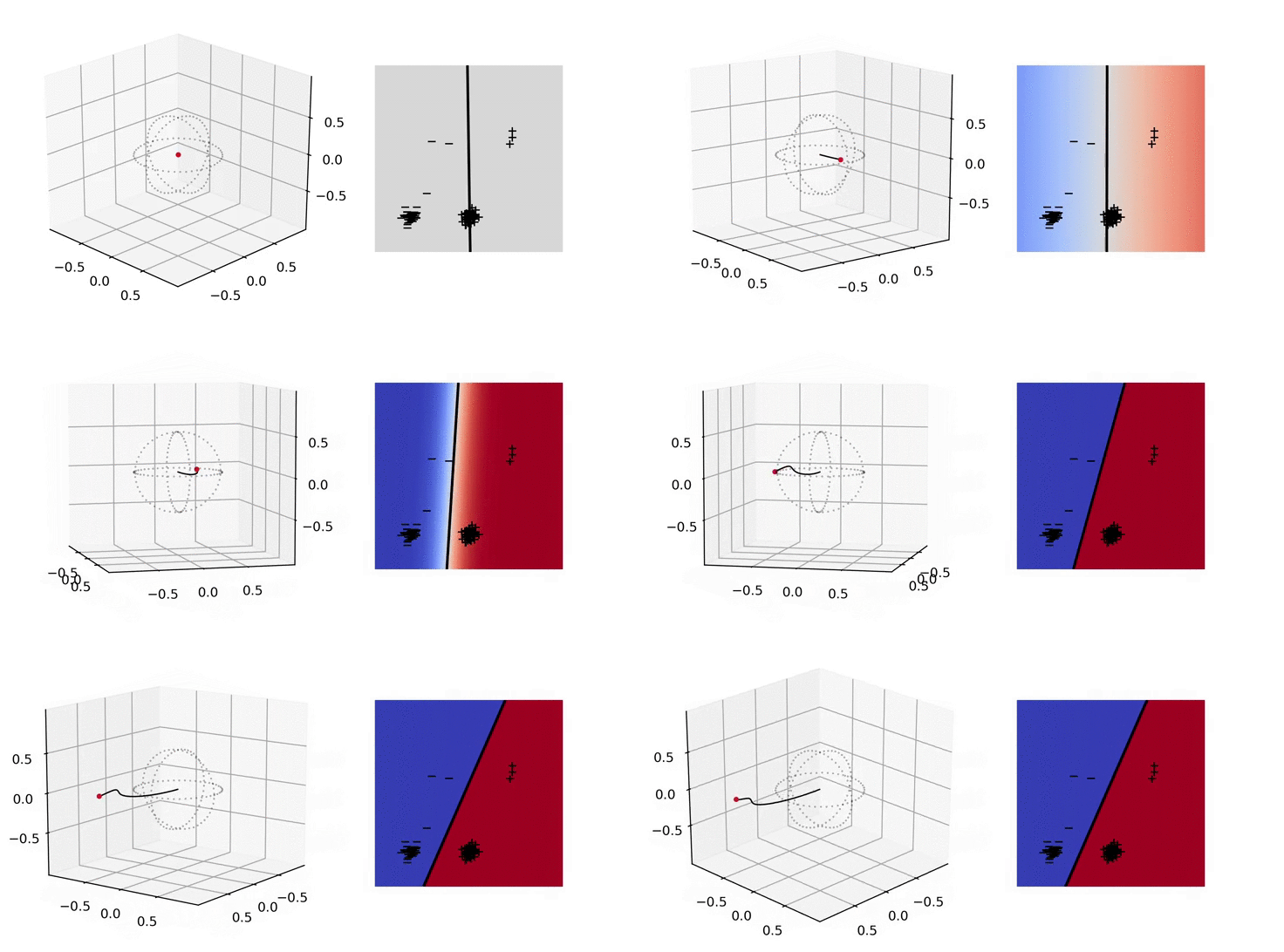
Illustration. In the figure below, we plot on the left the evolution of the parameter \(a(t)\) and on the right the predictor \(x\mapsto (x,1)^\top a(t)\) with \(x\in \mathbb{R}^2\). In parameter space, we apply the hyperbolic tangent to the radial component which allows to easily visualize diverging trajectories. This way, the unit sphere represents the horizon of \(\mathbb{R}^d\), i.e., the set of directions at infinity [Chap. 3 in 9]. We will use the same convention in the other plots below.

3. Implicit bias: training only the output layer

Despite its apparently restrictive setting, the previous result already tells us something about wide neural networks. Consider the situation touched upon earlier where we only train the output weights \(a_j\) and the hidden weights \(b_j\) are picked uniformly at random on the sphere. This corresponds to learning a linear classifier on top of the random feature \([(b_j^\top x)_+]_{j=1}^m\).

As we have just shown, if the training set is separable, the normalized gradient flow of the unregularized exponential loss (or logistic loss) converges to a solution to $$ \max_{\Vert a\Vert_2 \leq 1}\min_i y_i \sum_{j=1}^m a_j (b_j^\top x_i)_+.$$

This is a random feature approximation for the unregularized kernel support vector machine problem in the RKHS \(\mathcal{F}_2\), which is recovered in the large width limit \(m\to \infty\): $$\max_{\Vert h\Vert_{\mathcal{F}_2}\leq 1} \min_i y_i h(x_i).$$ Notice that if \(m\) is large enough, the linear separability assumption is not even needed anymore, because any training set is separable in \(\mathcal{F}_2\) (at least if all \(x_i\)s are distinct and if we do not forget to include the bias/intercept).

Illustration. In the animation below, we plot on the left the evolution of the parameters and on the right the predictor for a 2-D classification task. In parameter space, each particle represents a neuron: their direction is fixed, their distance to \(0\) is their absolute weight and the color is red (+) or blue (-) depending on the sign of the weight. As above, the unit sphere is at infinity and the particles diverge. In predictor space, the markers represent the training samples of both classes, the color shows the predictor and the black line is the decision boundary. The fact that the predictor has a smooth decision boundary is in accordance with the properties of \(\mathcal{F}_2\) given above.

4. Implicit bias: 2-homogeneous linear classifiers

Although the analyses where neural networks behave like kernel methods are pleasant for us theoreticians because we are in conquered territory, they miss essential aspects of neural networks such as their adaptivity and their ability to learn a representation. Let us see if we can characterize the implicit bias of the gradient flow of the unregularized exponential loss when training both layers of the neural network.

A 2-homogeneous linear model. From an optimization point of view, an important property of two layer relu neural networks is that \(\Phi(\alpha w)= \alpha^2 \Phi(w)\) for all \(\alpha>0\), i.e., they are positively 2-homogeneous in the training parameters. In contrast, a linear model is 1-homogeneous in the parameters. This seemingly little difference leads to drastic changes in the gradient flow dynamics.

Let us again build our intuition with a simplified model that captures key aspects of the dynamics, namely the linear classification setting of above. This time, we take any initialization \(r(0)\in \mathbb{R}^d\) with positive entries and the gradient flow in the ascent direction of the function \( F(r\odot r)\) where \(\odot\) is the elementwise product between two vectors and \(F\) is defined in Eq. (5). This is just a trick to obtain a 2-homogeneous parameterization of a linear model. This gradient flow satisfies $$ r'(t) = 2 r(t)\odot \nabla F(r(t)\odot r(t)).$$

Normalized dynamics. Let us define \(\bar a(t):=(r(t)\odot r(t))/\Vert r(t)\Vert_2^2\) the normalized predictor associated to our dynamics which, by definition, belongs to the simplex \(\Delta_d\), i.e., the set of nonnegative vectors in \(\mathbb{R}^d\) that sum to one. Using the fact that \(\nabla F(\beta a) = \nabla F_\beta (a)\) for all \(\beta>0\), we obtain $$\begin{aligned} \bar a'(t) &= 2\frac{r(t)\odot r'(t)}{\Vert r(t)\Vert_2^2} -2 (r(t)^\top r'(t))\frac{r(t)\odot r(t)}{\Vert r(t)\Vert_2^4}\\ &=4\bar a(t) \odot \nabla F_{\Vert r(t)\Vert_2^2}(\bar a(t))\ – \alpha(t) \bar a(t)\end{aligned}$$ where \(\alpha(t)\) is the scalar such that \(\sum_{i=1}^d a’_i(t) =0\). Online optimization experts might have recognized that this is (continuous time) online mirror ascent in the simplex for the sequence of smooth-margin functions \(F_{\Vert r(t)\Vert_2^2}\). Notice in particular the multiplicative updates: they correspond to the entropy mirror function, and they are particularly well suited for optimization in the high dimensional simplex [Chap.4, 14].

What do we learn from this reformulation?

• We can prove (by similar means) that if the data set is linearly separable then \(\Vert r(t)\Vert_2^2\) diverges. So the sequence of functions \(F_{\Vert r\Vert_2^2}\) converges to the margin \(F_\infty\) which means that \(\bar a(t)\) just ends up optimizing the function \(F_\infty\). As a consequence, we have $$\lim_{t\to \infty} y_i x_i^\top \bar a(t) = \max_{a\in \Delta_d} \min_{i} y_i x_i^\top a.$$ This exposes another implicit bias of gradient flow. Notice the key difference with the implicit bias obtained with a linear parameterization: we obtain here the \(\ell_1\)-max-margin (over classifiers with non-negative entries) instead of the \(\ell_2\)-max-margin.
• Beyond exposing the implicit bias, this reformulation shows that \(\bar a(t)\) implicitly optimizes a sequence of smooth objectives which converge to the margin \(F_\infty\). Unknowingly, we have recovered the well-principled optimization method that consists in approximating a non-smooth objective with smooth functions [15].
• While the conclusion above was only formal, this point of view leads to rigorous proofs of convergence and convergence rates in discrete time in \(\tilde O(1/\sqrt{t})\) with a step-size in \(O(1/\sqrt{t})\), by exploiting tools from online optimization, see [1].

5. Implicit bias: fully trained 2-layer neural networks

Once again this argument about linear predictors applies to neural networks: if we train both layers but only the magnitude of the hidden weights and not their direction, then this is equivalent to learning a 2-homogeneous linear model on top of the random feature \([ a_j(0) (x_i^\top b_j(0))_+]_{j=1}^m\). If each feature appears twice with opposite signs — which is essentially the case in the large width limit — then the simplex constraint can be equivalently replaced by an \(\ell_1\)-norm constraint on the weights. Recalling the definition of the \(\mathcal{F}_1\)-norm from Eq. (4), we thus obtain that, in the infinite-width limit, the normalized predictor converges to a solution to $$ \max_{\Vert h\Vert_{\mathcal{F}_1} \leq 1} \min_i y_i h(x_i).$$

This result is correct, but it is not relevant. In contrast to functions in \(\mathcal{F}_2\), functions in \(\mathcal{F}_1\) can not in general be approximated with few random features in high dimension. In fact, lower bounds that are exponential in the dimension exist in certain settings [Sec. X, 16]. They can be approximated with a small number of features but those need to be data-dependent: in that sense, it is necessary to learn a representation – here, a distribution over the hidden weights — in order to learn in \(\mathcal{F}_1\).

This raises the following question: do we obtain the same implicit bias when training both layers of the neural network, without fixing the direction of the input weights? In the following result, which is the main theorem of our paper [1], we answer by the affirmative.

Theorem (C. and Bach [1], informal). Assume that for some \(\sigma>0\), the hidden weights \(b_j\) are initialized uniformly on the sphere of radius \(\sigma\) and the output weights \(a_j\) are uniform in \(\{-\sigma,\sigma\}\). Let \(\mu_t\) be the Wasserstein gradient flow for the unregularized exponential loss and \(h_t = \int \Phi(w)d\mu_t(w)\) be the corresponding dynamics in predictor space. Under some technical assumptions, the normalized predictor \(h_t/\Vert h_t\Vert_{\mathcal{F}_1}\) converges to a solution to the \(\mathcal{F}_1\)-max-margin problem: $$\max_{\Vert h\Vert_{\mathcal{F}_1} \leq 1} \min_i y_i h(x_i).$$

Giving an idea of proof would be a bit too technical for this blog post, but let us make some remarks:

• The strength of this result is that although this dynamics could get trapped towards limit directions which are not optimal, this choice of initialization allows to avoid them all and to only converge to global minimizers of this max-margin problem. The principle behind this is similar to the global convergence result in the previous blog post.
• The fact that optimizing on the direction of the hidden weights is compatible with the global optimality conditions of the \(\mathcal{F}_1\)-max-margin problem is very specific to the structure of positively 2-homogeneous problems, and should not be taken for granted for other architectures of neural networks.
• Although at a formal level this result works for any initialization that is diverse enough (such as the standard Gaussian initialization), the initialization proposed here yields dynamics with a better behavior for relu networks: by initializing the hidden and output weights with equal norms – a property preserved by the dynamics – we avoid some instabilities in the gradient. Also notice that this result applies to any scale \(\sigma>0\) of the initialization (we’ll see an intriguing consequence of this in the next section).

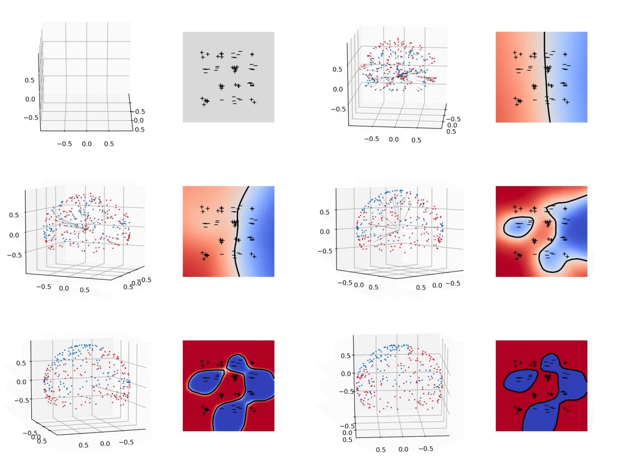
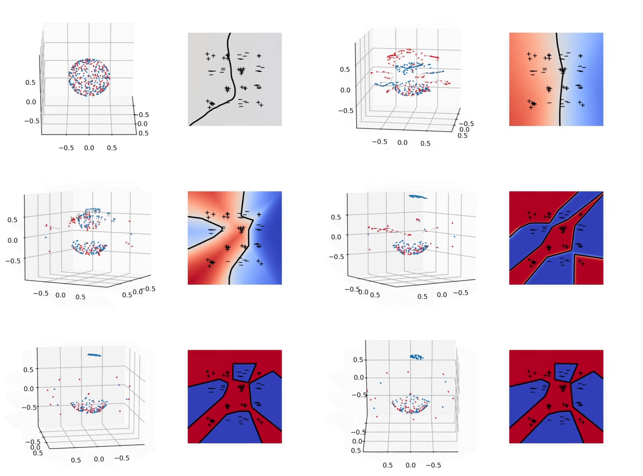
Illustration. In the figure below, we plot the training dynamics when both layers are trained. In parameter space (left), each particle represents a neuron: its position is \(\vert a_j\vert b_j\) and its color depends on the sign of \(a_j\). Here again the unit sphere is at infinity. The inactive neurons at the bottom correspond to those with a bias that is “too negative” at initialization. We observe that all the other neurons gather into few clusters: this is the sparsifying effect of the \(L^1\)-norm in Eq. (4). In predictor space, we obtain a polygonal classifier, as expected for a \(\mathcal{F}_1\)-max-margin classifier. See the paper [1] for experiments that illustrate the strengths of this classifier in terms of generalization.

6. Lazy regime and the neural tangent kernel

This blog post would not be complete without mentioning the lazy regime. This is yet another kind of implicit bias which, in our context, takes place when at initialization the weights have a large magnitude and the step-size is small. It was first exhibited in [17] for deep neural networks (see also [18, 19]). Hereafter, we follow the presentation of [20].

Lazy training via scaling. This phenomenon is in fact very general so let us present it with a generic parametric predictor \(h(W)\) with differential \(Dh(W)\). We introduce a scaling factor \(\alpha>0\) and look at the gradient flow of \(F(W) := R(\alpha h(W))\) with a step-size \(1/\alpha^2\), that is $$ W'(t) = \ – \frac{1}{\alpha}Dh(W(t))^\top \nabla R(\alpha h(W(t))),$$ with initialization \(W(0)\). In terms of the predictor \(\alpha h(W)\), this yields the dynamics $$\frac{d}{dt} \alpha h(W(t)) = \ – Dh(W(t))Dh(W(t))^\top \nabla R(\alpha h(W(t)).$$

Lazy training happens when we take \(\alpha\) large while making sure that \(\alpha h(W(0))\) stays bounded. In this case, we see that the parameters change at a rate \(O(1/\alpha)\), while the predictor changes at a rate independent of \(\alpha\). On any bounded time interval, in the limit of a large \(\alpha\), the parameters only move infinitesimally, while the predictor still makes significant progress, hence the name lazy training.

Equivalent linear model. Since the parameters hardly move, if we assume that \(Dh(W(0))\neq 0\) then we can replace the map \(h\) by its linearization \(W \mapsto h(W(0))+Dh(W(0))(W-W(0))\). This means that the training dynamics essentially follows the gradient flow of the objective $$ R\big ( \alpha h(W(0)) + \alpha Dh(W(0))(W-W(0)) \big)$$ which is a convex function of \(W\) as soon as \(R\) is convex.

If this objective admits a minimizer that is not too far away from \(W(0)\), then \(W(t)\) converges to this minimizer. If in contrast all the minimizers are too far away (think of the exponential loss where they are at infinity), then the parameters will eventually move significantly and the lazy regime is just a transient regime in the early phase of training. Of course, all these behaviors can be quantified and made more precise, because this phenomenon brings us back to the realm of linear models.

What all of this has to do with two-layer neural networks? As it happens, this scale factor appears implicit in various situations for these models; let us detail two of them.

Neural networks with \(1/\sqrt{m}\) scaling. For two-layer neural networks, lazy training occurs if we define \(h = \frac{1}{\sqrt{m}} \sum_{j=1}^m \Phi(w_j)\) instead of \(h=\frac{1}{m} \sum_{j=1}^m \Phi(w_j)\) before taking the infinite width limit. Indeed:

• This induces a scaling factor \(\alpha = \sqrt{m} \to \infty\) compared to \(1/m\) which, as we have already seen, is the “correct” scaling that leads to a non-degenerate dynamics in parameter space as \(m\) increases.
• Moreover, by the central limit theorem, \(\frac{1}{\sqrt{m}} \sum_{j=1}^m \Phi(w_j(0)) = O(1)\) for typical random initializations of the parameters. So the initial predictor stays bounded.

To take the Wasserstein gradient flow limit, the step-size has to be of order \(m\) (see previous blog post). So here we should take a step-size of order \(m/\alpha^2 = 1\). With such a step-size, all the conditions for lazy training are gathered when \(m\) is large. Intuitively, each neuron only moves infinitesimally, but they collectively produce a significant movement in predictor space.

Neural networks with large initialization. Coming back to our scaling in \(1/m\) and our Wasserstein gradient flow that is obtained in the large width limit, there is another way to enter the lazy regime: by increasing the variance of the initialization.

To see this, assume that \(h\) is a positively \(p\)-homogeneous parametric predictor, which means that \(h(\sigma W)=\sigma^p h(W)\) for all \(\sigma>0\) and some \(p>1\) (remember that this is true with \(p=2\) for our two-layer relu neural network). Take an initialization of the form \(W(0) = \sigma \bar W_0\) where \(\sigma>0\) and \(h(\bar W_0)=0\) (which is also satisfied for our infinite width neural networks with the initialization considered previously). Consider the gradient flow of \(R(h(W))\) with step-size \(\sigma^{2-2p}\). By defining \(\bar W(t) = W(t)/\sigma\) and using the fact that the differential of a p-homogeneous function is (p-1)-homogeneous, we have, on the one hand $$ \bar W'(t) = -\sigma^{-p} Dh(\bar W(t))^\top \nabla R(\sigma^p h(\bar W(t))), $$ and on the other hand $$\frac{d}{dt} \sigma^p h(\bar W(t)) =\ – Dh(\bar W(t))Dh(\bar W(t))^\top \nabla R(\sigma^p h(\bar W(t))).$$ So in terms of the dynamics \(\bar W(t)\), the situation is exactly equivalent to having a scaling factor \(\alpha=\sigma^p\). This implies that as the magnitude \(\sigma\) of the initialization increases, we enter the lazy regime, provided the step-size is of order \(\sigma^{2-2p}\).

Neural tangent kernel. What does the lazy regime tell us about the learnt predictor for two-layer neural networks? Assuming for simplicity that the predictor at initialization is \(0\), this regime amounts to learning a linear model on top of the feature \([(b_j^\top x)_+]_{j=1}^m\) — the derivative with respect to the output weights — concatenated with the feature \([x a_j 1_{b_j^\top x > 0} ]_{j=1}^m\) — the derivative with respect to the input weights. Compared to training only the output layer, this thus simply adds some features.

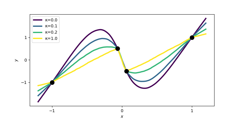
Assume for concreteness, that at initialization the hidden weights \(b_j\) are uniform on a sphere of large radius \(\sigma>0\) and the output weights are uniform on \(\{-\kappa\sigma, \kappa\sigma\}\) where \(\kappa\geq 0\). For a large width and a large \(\sigma\), we enter the lazy regime which amounts to learning in a RKHS — let us call it \(\mathcal{F}_{2,\kappa}\) — that is slightly different from \(\mathcal{F}_2 = \mathcal{F}_{2,0}\), since its kernel \(K_\kappa\) contains another term: $$ K_\kappa(x,x’) = \int_{\mathbb{S}^{d-1}} (\theta^\top x)_+ (\theta^\top x’)_+d\tau(\theta) + \kappa^2 \int_{\mathbb{S}^{d-1}} (x^\top x’) 1_{\theta^\top x > 0}1_{\theta^\top x’ > 0}d\tau(\theta). $$

This kernel is called the Neural Tangent Kernel [17] and the properties of the associated RKHS have been studied in [21, 22], where it is shown to include functions that are slightly less smooth than those of \(\mathcal{F}_2\) when \(\kappa\) increases. This is illustrated in the plot below, obtained by training a wide neural network with \(\sigma\) large (to reach the lazy regime) on the square loss, and various values of \(\kappa\).

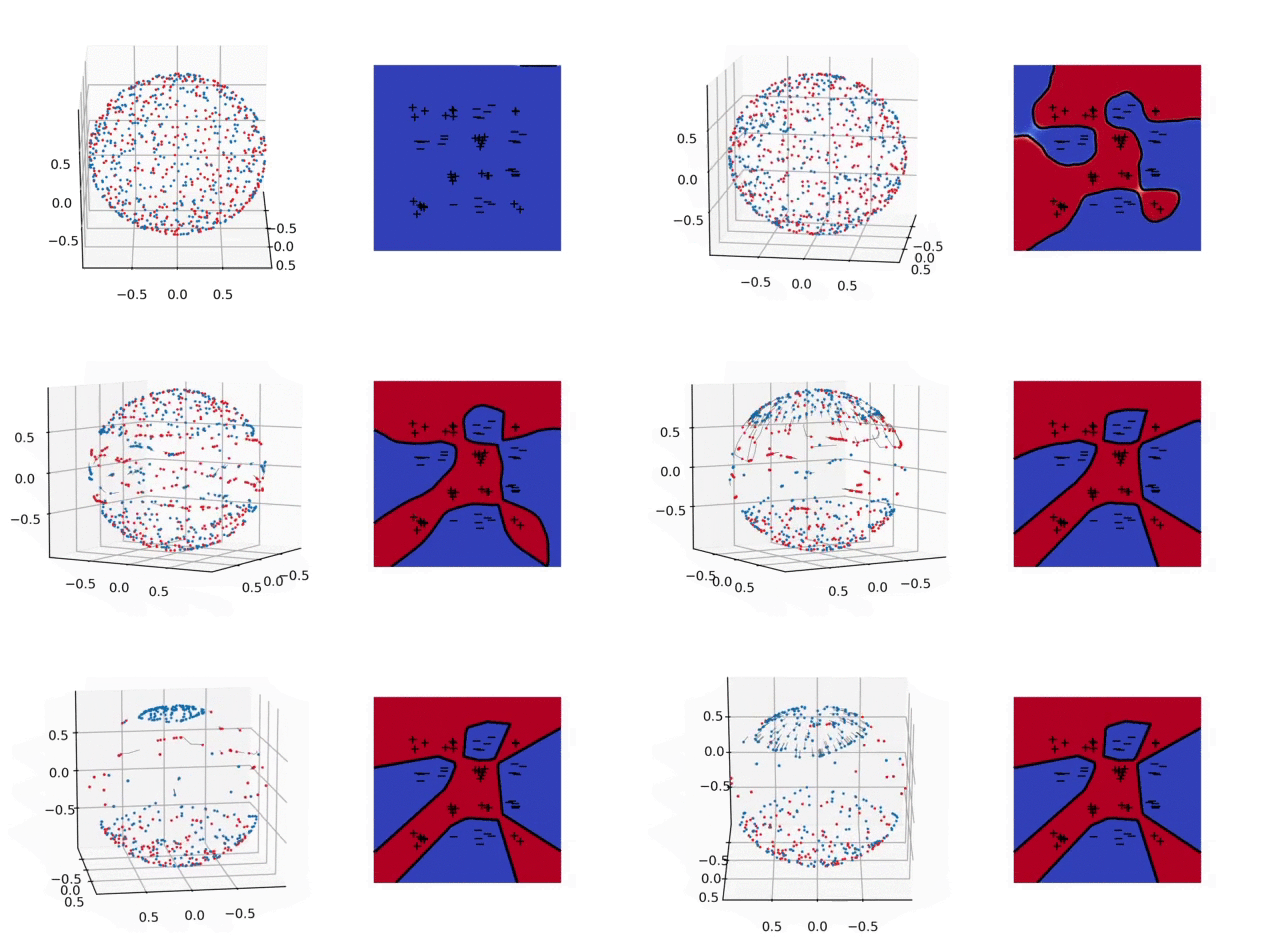
Two implicit biases in one shot. The attentive reader might have noticed that for large initialization scale \(\sigma\gg 1\), when training both layers on the unregularized exponential loss, two of our analyses apply: lazy training — that leads to a max-margin predictor in \(\mathcal{F}_{2,\kappa}\) — and the asymptotic implicit bias — that leads to a max-margin predictor in \(\mathcal{F}_{1}\). So, where is the catch?

There is none! Since the minimizers of this loss are at infinity, the lazy regime is just a transient phase and we will observe both implicit biases along the training dynamics! Take a look at the video below: we observe that in early phases of training, the neurons do not move while learning a smooth classifier — this is the lazy regime and the classifier approaches the \(\mathcal{F}_{2,\kappa}\)-max-margin classifier. In later stages of training, the neurons start moving and the predictor converges to a \(\mathcal{F}_1\)-max-margin classifier as stated by the main theorem. The predictor jitters a little bit during training because I have chosen rather aggressive step-sizes. As shown in [23], the transition between these two implicit biases can be well understood in some simpler models.

Discussion

In this blog post, I described how analyses of the training dynamics can help us understand the properties of the predictor learnt by neural networks even in the absence of an explicit regularization. Already for the simplest algorithm one can think of — gradient descent — we have found a variety of behaviors depending on the loss, the initialization or the step-size.

To achieve this description, the infinite width limit is of great help. It allows to obtain synthetic and precise characterizations of the learnt predictor, that can be used to derive generalization bounds. Yet, there are many interesting non-asymptotic effects caused by having a finite width. In that sense, we were only concerned with the end of the curve of double descent [24].

References

[1] Lénaïc Chizat, Francis Bach. Implicit Bias of Gradient Descent for Wide Two-layer Neural Networks Trained with the Logistic Loss. To appear in Conference On Learning Theory, 2020.
[2] Francis Bach. Breaking the curse of dimensionality with convex neural networks. The Journal of Machine Learning Research, 18(1), 629-681, 2017.
[3] Vera Kurková, Marcello Sanguineti. Bounds on rates of variable-basis and neural-network approximation. IEEE Transactions on Information Theory, 47(6):2659-2665, 2001.
[4] Behnam Neyshabur, Ryota Tomioka, Nathan Srebro. In Search of the Real Inductive Bias: On the Role of Implicit Regularization in Deep Learning. ICLR (Workshop). 2015.
[5] Youngmin Cho, Lawrence K. Saul. Kernel methods for deep learning. Advances in neural information processing systems. 342-350, 2009.
[6] Radford M. Neal. Bayesian learning for neural networks. Springer Science & Business Media, 2012.
[7] Ali Rahimi, Benjamin Recht. Random features for large-scale kernel machines. Advances in neural information processing systems. 1177-1184, 2008.
[8] Kevin P. Murphy. Machine Learning: A Probabilistic Perspective. The MIT Press, 2012
[9] Daniel Soudry, Elad Hoffer, Mor Shpigel Nacson, Suriya Gunasekar, Nathan Srebro. The Implicit Bias of Gradient Descent on Separable Data. The Journal of Machine Learning Research, 19(1), 2822-2878, 2018.
[10] R. Tyrrell Rockafellar, Roger J-B. Wets. Variational analysis. Springer Science & Business Media, 2009.
[11] Suriya Gunasekar, Jason D. Lee, Daniel Soudry, Nathan Srebro. Characterizing implicit bias in terms of optimization geometry. International Conference on Machine Learning, 2018.
[12] Ziwei Ji, Matus Telgarsky. Risk and parameter convergence of logistic regression. 2018.
[13] Matus Telgarsky. Margins, Shrinkage, and Boosting. International Conference on Machine Learning, 307-315, 2013.
[14] Sébastien Bubeck. Convex Optimization: Algorithms and Complexity. Foundations and Trends in Machine Learning, 8(3-4):231-357, 2015.
[15] Yuri Nesterov. Smooth minimization of non-smooth functions. Mathematical programming, 103(1):127-152, 2005.
[16] Anrew R. Barron. Universal approximation bounds for superpositions of a sigmoidal function. IEEE Transactions on Information theory. 39(3), 930-945, 1993.
[17] Arthur Jacot, Franck Gabriel, Clément Hongler. Neural tangent kernel: Convergence and generalization in neural networks. Advances in neural information processing systems. 8571-8580, 2018.
[18] Simon S Du, Xiyu Zhai, Barnabas Poczos, Aarti Singh. Gradient descent provably optimizes over-parameterized neural networks. International Conference on Learning Representations. 2019.
[19] Zeyuan Allen-Zhu, Yuanzhi Li, Zhao Song. A Convergence Theory for Deep Learning via Over-Parameterization. International Conference on Machine Learning, PMLR 97:242-252, 2019.
[20] Lénaïc Chizat, Édouard Oyallon, Francis Bach. On lazy training in differentiable programming. Advances in Neural Information Processing Systems. 2937-2947, 2019.
[21] Behrooz Ghorbani, Song Mei, Theodor Misiakiewicz, Andrea Montanari. Linearized two-layers neural networks in high dimension. To appear in Annals of Statistics. 2019.
[22] Alberto Bietti, Julien Mairal. On the Inductive Bias of Neural Tangent Kernels. Advances in Neural Information Processing Systems. p. 12893-12904, 2019.
[23] Edward Moroshko, Suriya Gunasekar, Blake Woodworth, Jason D. Lee, Nathan Srebro, Daniel Soudry. Implicit Bias in Deep Linear Classification: Initialization Scale vs Training Accuracy. Technical report arXiv:2007.06738, 2020.
[24] Mikhail Belkin, Daniel Hsu, Siyuan Ma, Soumik Mandal. Reconciling modern machine-learning practice and the classical bias–variance trade-off. Proceedings of the National Academy of Sciences. 116(32), 15849-15854, 2019.

Lower bound on the gradient norm for linear classification with the exponential loss

In the context of Section 2, we want to prove that \(\Vert \nabla F(a)\Vert_2\geq \gamma\). For this, let \(Z\in \mathbb{R}^{n\times d}\) be the matrix with rows \(y_i x_i\) and let \(\Delta_n\) be the simplex in \(\mathbb{R}^n\). We have by duality $$ \gamma = \max_{\Vert a\Vert_2\leq 1}\min_{p\in \Delta_n} p^\top Z a = \min_{p\in \Delta_n} \max_{\Vert a\Vert_2\leq 1} a^\top Z^\top p = \min_{p\in \Delta_n} \Vert Z^\top p\Vert_2 .$$ Also, notice that \(\nabla F(a) = Z^\top p\) with \(p_i = \frac{e^{-y_ix_i^\top a}}{\sum_{j=1}^n e^{-y_{j}x_{j}^\top a}}\). Since \(p \in \Delta_n\), we conclude that \(\Vert \nabla F(a)\Vert_2\geq \min_{p\in \Delta_n} \Vert Z^\top p\Vert_2 = \gamma\).