Gradient descent for wide two-layer neural networks – I : Global convergence

Supervised learning methods come in a variety of flavors. While local averaging techniques such as nearest-neighbors or decision trees are often used with low-dimensional inputs where they can adapt to any potentially non-linear relationship between inputs and outputs, methods based on empirical risk minimization are the most commonly used in high-dimensional settings. Their principle is simple: optimize the (potentially regularized) risk on training data over prediction functions in a pre-defined set of functions.

When the set of a functions is a convex subset of a vector space with a finite-dimensional representation, with standard assumptions, the corresponding optimization problem is convex. This has the benefits of allowing a thorough theoretical understanding of the computational and statistical properties of learning methods, which often come with strong theoretical guarantees, in terms of running time [1, 2, 3] or prediction performance on unseen data [4, 5]. In particular, the linear parameterization can be done either explicitly by building a typically large finite set of features, or implicitly through the use of kernel methods and then a series of dedicated algorithms and theories can be leveraged for efficient non-linear predictions [6, 7, 8].

However, linearly-parameterized sets of functions do not include neural networks, which lead to state-of-the-art performance in most learning tasks in computer vision, natural language processing, speech processing, in particular through the use of deep and convolutional neural networks [9].

Two-layer neural networks with “relu” activations

The goal of this blog post is to provide some understanding of why supervised machine learning work for the simplest form of such models: $$ h(x) = \frac{1}{m} \sum_{i=1}^m a_i ( b_i^\top x)_+ = \frac{1}{m} \sum_{i=1}^m a_i \max\{ b_i^\top x,0\},$$ where the input \(x\) is a vector in \(\mathbb{R}^d\), and \(m\) is the number of hidden neurons. The weights \(a_i \in \mathbb{R}\), \(i=1,\dots,m\), are the output weights, while the weights \(b_i \in \mathbb{R}^d\), \(i=1,\dots,m\), are the input weights. The rectified linear unit (“relu”) [10] activation is used, and our results will depend heavily on its positive homogeneity (that is, for \(\lambda > 0\), \((\lambda u)_+ = \lambda u_+\)).

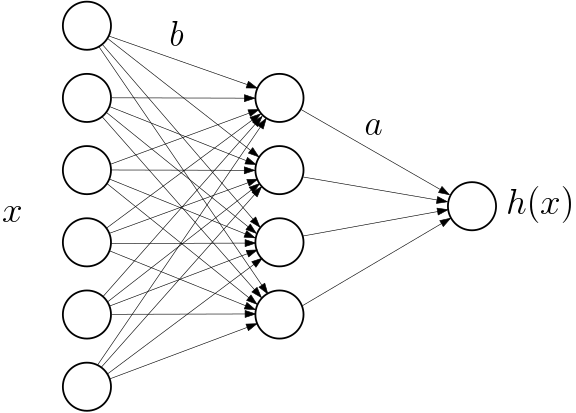
Note that this is an idealized and much simplified set-up for deep learning, as there is a single hidden-layer, no convolutions, no pooling, etc. As I will show below, this simple set-up is already complex to understand, and I believe it captures some of the core difficulties associated with non-convexity.

The first question that one may come to after decades of research in learning theory is: why is it so hard to analyze?

There are at least two major difficulties:

• Non-linearity: the dependence on the input weights \(b_i\)’s is non-linear because of the activation function, typically leading to non-convex optimization problems.
• Overparameterization: The number \(m\) of hidden neurons is very large (often so large that the number of parameters \(m(d+1)\) exceeds the number of observations), which is hard in terms of optimization and potentially generalization to unseen data.

In this blog post, we will leverage the overparameterization and take \(m\) tending to infinity (without any dependence on the number of observations), which will allow us to derive theoretical results. We will leverage two key properties of the problem:

• Separability of the model in \(w_i = (a_i,b_i)\), that is, the prediction function \(h(x)\) is the sum of terms which are independently parameterized, as \(h = \frac{1}{m} \sum_{i=1}^m \Phi(w_i)\), where \(\Phi: \mathbb{R}^p \to \mathcal{F}\), with \(\mathcal{F}\) a space of functions. In our situation, \(p = d+1\) and: $$ \Phi(w)(x) = a (b^\top x)_+. $$ In other words, there is no parameter sharing among hidden neurons. Unfortunately, this does not generalize to more than a single hidden layer.
• Homogeneity: the relu activation is positively homogeneous so that as as function of \(w = (a,b) \in \mathbb{R} \times \mathbb{R}^d\), \(\Phi(w)(x) = a (b^\top x)_+\) is positively 2-homogeneous, that is, \(\Phi(\lambda w) = \lambda^2 \Phi(w)\) for \(\lambda > 0\).

In this sequence of two blog posts, following a recent trend in optimization and machine learning theory [11, 12], optimization and statistics cannot be separated and need to be tackled together. I will focus on gradient flows on empirical or expected risks.

In this blog post, I will cover optimization and how over-parameterization leads to global convergence for 2-homogeneous models, a recent result obtained two years ago with Lénaïc Chizat [13]. This requires tools from optimal transport which I will briefly describe (for more details, see, e.g., [14]).

Next month, I will focus on generalization capabilities and the several implicit biases associated with gradient descent in this context [15, 16].

Infinitely wide limit and probability measures

Following the standard learning set-up, our goal will be to minimize with respect to the prediction function \(h\) the functional \(R\) defined as $$ R(h) = \mathbb{E}_{p(x,y)} \big[ \ell( y, h(x) ) \big],$$ where \(\ell(y,h(x))\) is the loss incurred by outputting \(h(x)\) when \(y\) is the true label. Even within deep learning, this loss is most often convex in its second argument, such as for least-squares or logistic losses. Thus, I will assume that \(R\) is convex.

The expectation can be considered in two scenarios:

• Empirical risk: this corresponds to the situation where we have observations \((x_j,y_j)\), \(j=1,\dots,n\), coming from some joint distribution on \((x,y) \in \mathbb{R}^d \times \mathbb{R}\). Minimizing \(R\) then may not lead to any guarantee on unseen data unless some explicit or implicit regularization is used. In next blog post, I will consider the implicit regularization effect of gradient-based algorithms.
• Expected risk (or generalization performance): The expectation is taken with respect to unseen data, and thus its value (or a gradient) cannot be computed. However, any training observation \((x_j,y_j)\) can lead to an unbiased estimate, and if single pass stochastic gradient is used, our guarantees will be on the expected risk.

The main and very classical idea is to consider the minimization of $$ G(W) = G(w_1,\dots,w_m) = R \Big( \frac{1}{m} \sum_{i=1}^m \Phi(w_i) \Big),$$ and see it as the minimization of $$ F(\mu) = R \Big( \int_{\mathbb{R}^p} \Phi(w) d\mu(w) \Big),$$ with respect to a probability measure \(\mu\), with the equivalence for $$ \mu = \frac{1}{m} \sum_{i=1}^m \delta(w_i),$$ where \(\delta(w_i)\) is the Dirac measure at \(w_i\). See an illustration below.

When \(m\) is large, we can represent any measure in the weak sense (that is, expectations of any continuous and bounded functions can be approximated). The benefits of considering the space of all measures instead of discrete measures have been used already in variety of contexts in machine learning, statistics and signal processing [17, 18, 19]. In this blog post, the key benefit is that the set of measures in convex and \(h = \int_{\mathbb{R}^p} \Phi(w) d\mu(w) \) is linear in the measure \(\mu\), so that our optimization problem has become convex.

However, (1) It does not buy much in practice, as the set of probability measures is infinite-dimensional. Frank-Wolfe algorithms can be used, but the choice of new neurons is a difficult optimization problem, NP-hard for the threshold activation function [20], with polynomial potentially high complexity for the relu activation [21], and (2) this is not what is used in practice, which is (stochastic) gradient descent.

Finite-dimensional gradient flow

In this post, I will consider the gradient flow $$\dot{W} = \ – m \nabla G(W),$$ (where \(m\) is added as a normalization factor to allow a well-defined limit when \(m\) tends to infinity). This is still not exactly what is used in practice, but, as explained in last month post, this is a good approximation of gradient descent (if using the empirical risk, then leading to guarantees of global convergence on the empirical risk only), or stochastic gradient descent (if doing a single pass on the data, then leading to guarantees of global convergence on unseen data). This is a non-convex dynamics, with stationary points and local minima, even when \(m\) is large (see, e.g., [27]).

Two main questions arise: (1) what does the gradient flow dynamics converge to when the number of neurons \(m\) tends to infinity, and (2) can we get any global convergence guarantees for the limiting dynamics?

Mean-field limit and Wasserstein gradient flows

When \(m\) tends to infinity, since we want to use the measure representation, we need to understand the effect of performing the gradient flow jointly on \(w_1,\dots,w_m\) on the measure $$ \mu = \frac{1}{m} \sum_{i=1}^m \delta(w_i),$$ and see if we can take a limit when \(m\) tends to infinity. This process of taking limits is common in physics and often referred to as the “mean-field” limit, and has been considered in a series of recent works [22, 13, 23, 24]. To avoid too much technicality, I will assume that the map \(\Phi\) is sufficiently differentiable, which unfortunately exclude the relu activation; for dedicated results, see [13].

Gradient flows on metric spaces. In order to understand the dynamics in the space of probability measures, we need to take a step backward and realize that gradient flows can be defined for many functions \(f\) on any metric space \(\mathcal{X}\). Indeed, it can be seen as the limit of taking infinitesimal steps of length \(\gamma\), where each new iterate \(x_{k+1}\) (corresponding to the value at time \(k\gamma\)) is defined recursively from \(x_k\) as $$x_{k+1} \in \arg\min_{x \in \mathcal{X}}\ f(x) + \frac{1}{2\gamma} d(x,x_k)^2.$$ As shown in [25, 26], with some form of interpolation, this defines a curve with prescribed values \(x_k\) at each \(\gamma k\), and when the step-size \(\gamma\) goes to zero, this curves “converges” to the gradient flow.

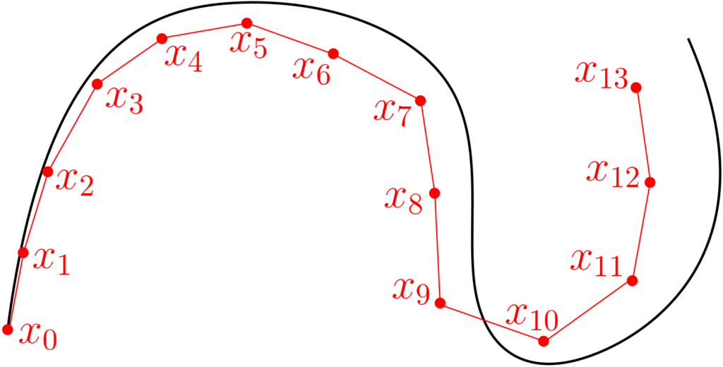
For the space \(\mathcal{X} = \mathbb{R}^d\) with the Euclidean distance and a continuously differentiable function \(f\), we obtain that $$x_{k+1} = x_k – \gamma f'(x_k) + o(\gamma),$$ and we get the usual gradient flow associated to \(f\), and the scheme above is nothing less than Euler discretization that was described last month.

Vector space gradient flows on probability measures. Probability measures are a convex subset of measures with finite total variation, which is equal to the \(\ell_1\)-norm between densities when the two probability measures have densities with respect to the same base measure. It is a normed vector space for which we could derive our first type of gradient flow, which can be seen as a continuous version of Frank-Wolfe algorithm, where atoms are added one by one, until convergence.

As mentioned above, the fact that atoms are created sequentially seems attractive computationally. However, (1) deciding which one to add is a computationally hard problem, and (2) the flow on measures cannot be approximated by a finite evolving set of “particles” (here hidden neurons each defined by a vector \(w \in \mathbb{R}^{d+1}\)).

Wasserstein gradient flows on probability measures. There is another natural distance here, namely the Wasserstein distance (sometimes called the Kantorovich–Rubinstein distance). In order to remain short, I will only define it between empirical measures $$\mu = \frac{1}{m} \sum_{i=1}^m \delta(w_i) \mbox{ and } \nu = \frac{1}{m} \sum_{i=1}^m \delta(v_i)$$ with the same number of points. The squared 2-Wasserstein distance is obtained by minimizing $$\frac{1}{m} \sum_{i=1}^m \| w_j – v_{\sigma(j)} \|_2^2$$ over all permutations \(\sigma: \{1,\dots,m\} \to \{1,\dots,m\}\). See illustration below.

This can be extended to any pair of probability measures, and used within gradient flows, it has a very natural decoupling property: if \(\mu\) is fixed, and \(\nu\) is within a small distance of \(\mu\) in Wasserstein distance, then the optimal permutation above will always be the same, that is, locally, the Wasserstein distance is a sum of squared Euclidean distances. Then, the Wasserstein gradient flow will lead to \(m\) independent local regular Euclidean gradient flows, which interact through the gradient term as: $$ \dot{w}_i = \ – \nabla \Phi(w_i) \nabla R\Big(\int_{\mathbb{R}^p} \Phi d\mu \Big),$$ where the Jacobian \(\nabla \Phi(w_i)\) is a linear operator from \(\mathcal{F}\) to \(\mathbb{R}^p\), and \( \nabla R: \mathbb{R}^p \to \mathcal{F}\) the gradient operator of \(R\). Since \(\mu = \frac{1}{m} \sum_{i=1}^m \delta(w_i)\), the dynamics of each particle interacts through the gradient of \(R\).

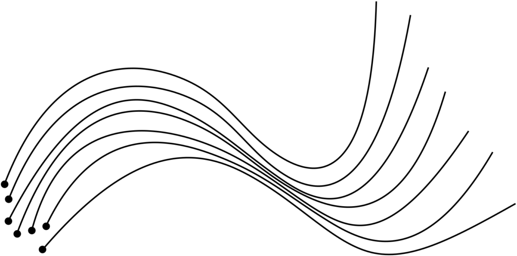
The intuitive reasoning above is behind the formal result for the function $$ F(\mu) = R \Big( \int_{\mathbb{R}^p} \Phi(w) d\mu(w) \Big),$$ that the limit of the Euclidean gradient flow on each particle when \(m\) tends to infinity, is exactly the Wasserstein gradient flow of \(F\). While I have proposed an intuitive explanation, this can be made more formal in particular through the use of partial differential equations on the density of the measure [13] (see also nice slides from Katy Craig on Wasserstein gradient flows).

Stationary points. Since \(R\) is assumed convex over the convex set of probability measures, all local minima of \(R\) are global, and we should expect the gradient flow to converge to global optimum from any initial measure. This is true for the gradient flow associated with the total variation metric. However this is not true for the Wasserstein gradient flow, for which stationary points which are not global minimizers exist (given that for discrete measures this corresponds to classical backpropagation, this is well known to anybody who has ever trained a neural network). Note that there exists a notion of convexity for Wasserstein gradient flows, namely geodesic convexity, but the function \(F\) is not geodesically convex in general.

Global convergence

We can now describe the main result from our recent work with Lénaïc [13]: under assumptions described below, for the function \(F\) defined above, if the Wasserstein gradient flow converges to a measure, this measure has to be a global minimum of \(F\) (note that we cannot prove it is always convergent).

On top of technical regularity assumptions that I will not describe here, we need two crucial broad assumptions:

• Homogeneity of the function \(\Phi: \mathbb{R}^{d+1} \to \mathcal{F}\). We need a condition of this form, since if \(R\) is a linear function, then \(F(\mu)\) is of the form \(F(\mu) = \int_{\mathbb{R}^p} \psi(w)d\mu(w)\) with \(\psi(w) = R(\Phi(w))\), and the Wasserstein gradient flow will converge to a weighted some of Diracs at all local minimizers of \(\psi\), which is typically not a global minimizer.
• Initialization with positive mass in all directions. That is, \(w_i\)’s are uniformly distributed on the sphere or Gaussian, which is the de facto choice in practice.

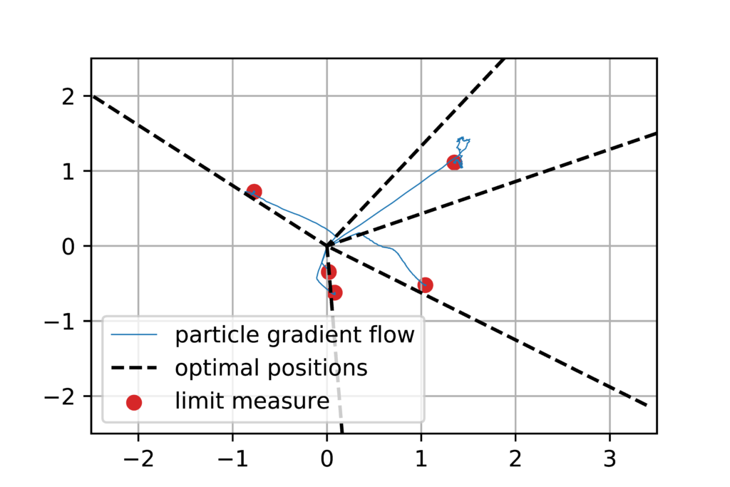
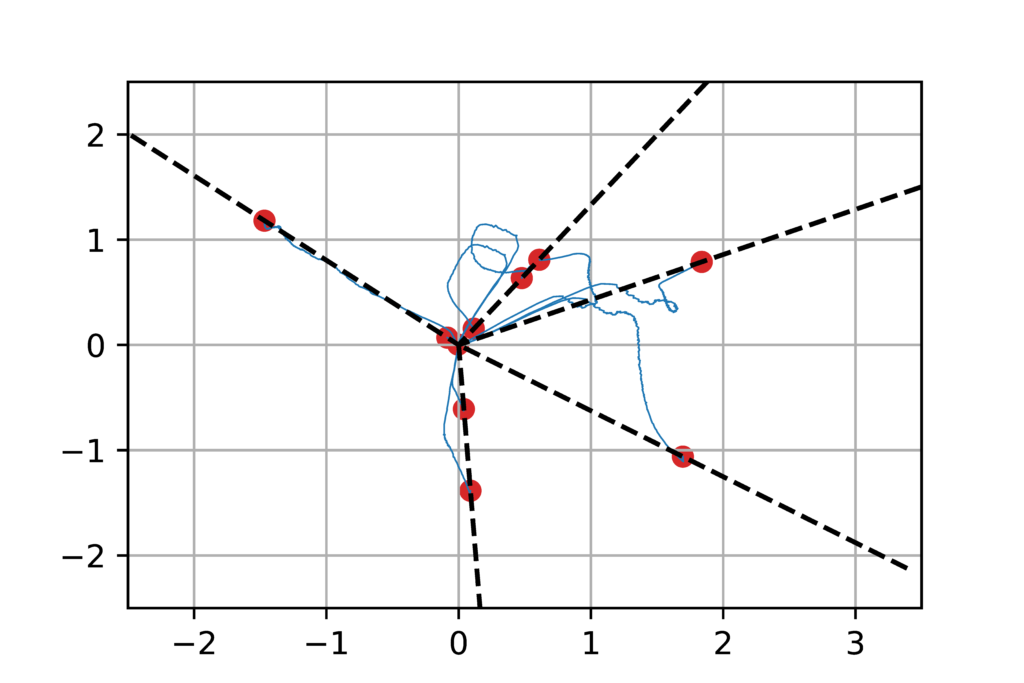
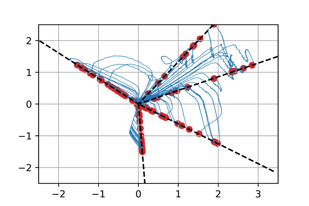
Illustration. We illustrate the result above by considering \(R\) as the square loss and \(y\) being generated from \(x\) through a neural network with \(m_0=5\) neurons. When running the gradient flow above, as soon as \(m \geqslant 5\), the model is sufficiently flexible to attain zero loss, which is thus the global optimum of the cost function. However, the gradient flow may not reach it, as it gets trapped in a local optimum. Our theoretical result suggests that when \(m\) is large, we should converge to the original neurons, which we see below. The surprising (and still unexplained) phenomenon is that \(m\) does not need to be much larger than \(m_0\) to see practical global convergence.

Discussion and open problems

In this blog post, I described theoretical results showing the benefits of overparameterization: when the number of hidden neurons \(m\) tends to infinity, then the corresponding gradient flow converges to the global optimum of the cost function. The proof relies notably on homogeneity properties of the relu activation.

The main weakness of this result is that is only qualitative: we cannot quantify how big \(m\) need to be to be close to the infinite width limit, or how fast the gradient flow converges to the global optimum. These are still open problems. Additional interesting areas of research are to extend these results to convolutional and/or deep networks.

Now that we know that we can obtain global convergence, I will describe next month the generalization properties when interpolating the training data with an overparameterized relu network [16].

Acknowledgements. I would like to thank Lénaïc Chizat for producing the nice figures and video of neural networks, proofreading this blog post, and making good clarifying suggestions.

References

[1] Sébastien Bubeck. Convex Optimization: Algorithms and Complexity. Foundations and Trends in Machine Learning, 8(3-4), 231-357, 2015.
[2] Léon Bottou, Frank E. Curtis, Jorge Nocedal. Optimization methods for large-scale machine learning. SIAM Review, 60(2):223-311, 2018.
[3] Francis Bach, Rodolphe Jenatton, Julien Mairal, Guillaume Obozinski. Optimization with sparsity-inducing penalties. Foundations and Trends in Machine Learning, 4(1):1-106, 2012.
[4] Shai Shalev-Shwartz, Shai Ben-David. Understanding machine learning: From theory to algorithms. Cambridge University Press, 2014.
[5] Larry Wasserman. All of statistics: a concise course in statistical inference. Springer Science & Business Media, 2013.
[6] Bernhard Schölkopf, Alexander J. Smola. Learning with kernels: support vector machines, regularization, optimization, and beyond. MIT press, 2002.
[7] Ali Rahimi and Benjamin Recht. Random features for large-scale kernel machines. Advances in neural information processing systems, 2008.
[8] Alessandro Rudi, Luigi Carratino, Lorenzo Rosasco. Falkon: An optimal large scale kernel method. Advances in Neural Information Processing Systems, 2017.
[9] Ian Goodfellow, Yoshua Bengio, Aaron Courville. Deep learning. MIT Press, 2016.
[10] Xavier Glorot, Antoine Bordes, and Yoshua Bengio. Deep sparse rectifier neural networks. International Conference on Artificial Intelligence and Statistics, 2011.
[11] Francis Bach and Eric Moulines. Non-strongly-convex smooth stochastic approximation with convergence rate O(1/n). Advances in Neural Information Processing Systems, 2013.
[12] MIkhail Belkin, Daniel Hsu, Siyuan Ma, Soumik Mandal. Reconciling modern machine-learning practice and the classical bias–variance trade-off. Proceedings of the National Academy of Sciences, 116(32), 15849-15854, 2019.
[13] Lénaïc Chizat, Francis Bach. On the Global Convergence of Gradient Descent for Over-parameterized Models using Optimal Transport. Advances in Neural Information Processing Systems, 2018.
[14] Gabriel Peyré, Marco Cututi. Computational Optimal Transport. Foundations and Trends in Machine Learning, 51(1):1–44, 2019.
[15] Lénaïc Chizat, Edouard Oyallon, Francis Bach. On Lazy Training in Differentiable Programming. Advances in Neural Information Processing Systems, 2019.
[16] Lénaïc Chizat, Francis Bach. Implicit Bias of Gradient Descent for Wide Two-layer Neural Networks Trained with the Logistic Loss. Technical report, arXiv:2002.04486, 2020.
[17] Andrew R. Barron. Universal approximation bounds for superpositions of a sigmoidal function. IEEE Transactions on Information theory, 39(3), 930-945, 1993.
[18] Yoshua Bengio, Nicolas Le Roux, Pascal Vincent, Olivier Delalleau, Patrice Marcotte. Convex neural networks. Advances in neural information processing systems, 2006.
[19] Francis Bach. Breaking the Curse of Dimensionality with Convex Neural Networks. Journal of Machine Learning Research, 18(19):1-53, 2017.
[20] Venkatesan Guruswami, Prasad Raghavendra. Hardness of learning halfspaces with noise. SIAM Journal on Computing, 39(2):742-765, 2009.
[21] Surbhi Goel, Varun Kanade, Adam Klivans, Justin Thaler. Reliably Learning the ReLU in Polynomial Time. Conference on Learning Theory, 2017.
[22] Atsushi Nitanda, Taiji Suzuki. Stochastic particle gradient descent for infinite ensembles. Technical report, arXiv:1712.05438, 2017.
[23] Song Mei, Andrea Montanari, Phan-Minh Nguyen. A mean field view of the landscape of two-layer neural networks. Proceedings of the National Academy of Sciences 115(33):E7665-E7671, 2018.
[24] Grant M. Rotskoff, Eric Vanden-Eijnden. Neural networks as interacting particle systems: Asymptotic convexity of the loss landscape and universal scaling of the approximation error. Technical report, arXiv:1805.00915, 2018.
[25] Luigi Ambrosio, Nicola Gigli, Giuseppe Savaré. Gradient flows: in metric spaces and in the space of probability measures. Springer Science & Business Media, 2008
[26] Filippo Santambrogio. {Euclidean, metric, and Wasserstein} gradient flows: an overview. Bulletin of Mathematical Sciences, 7(1), 87-154, 2017.
[27] Itay Safran, Ohad Shamir. Spurious Local Minima are Common in Two-Layer ReLU Neural Networks. International Conference on Machine Learning, 2018.