Effortless optimization through gradient flows

Optimization algorithms often rely on simple intuitive principles, but their analysis quickly leads to a lot of algebra, where the original idea is not transparent. In last month post, Adrien Taylor explained how convergence proofs could be automated. This month, I will show how proof sketches can be obtained easily for algorithms based on gradient descent. This will be done using vanishing step-sizes that lead to gradient flows.

Gradient as local information

The intuitive principle behind gradient descent is the quest for local descent. We thus need to characterize the local behavior of the function we aim to optimize. This is what gradients are for.

In this blog post, I will consider minimizing a function \(f\) over \(\mathbb{R}^d\). Assuming \(f\) is differentiable, a first order Taylor expansion of \(f\) around a point \(x\) leads to $$f(x+\delta) = f(x) + \nabla f(x) ^\top \delta + o(\| \delta\|),$$ for any norm \(\| \cdot \|\) on \(\mathbb{R}^d\), where \(\nabla f(x) \in \mathbb{R}^d\) is the gradient of \(f\) at \(x\), composed of partial derivatives of \(f\). Therefore, around \(x\), \(f\) is approximately affine.

Since we have a local affine approximation around \(x\), we can look for the direction of steepest descent, that is, the unit norm vector \(u \in \mathbb{R}^d\) such that \(f\) decays the most along \(u\), that is such that $$ u^\top \nabla f(x)$$ is minimized. This steepest descent direction depends on the choice of norm (assuming that the gradient is not zero at \(x\)).

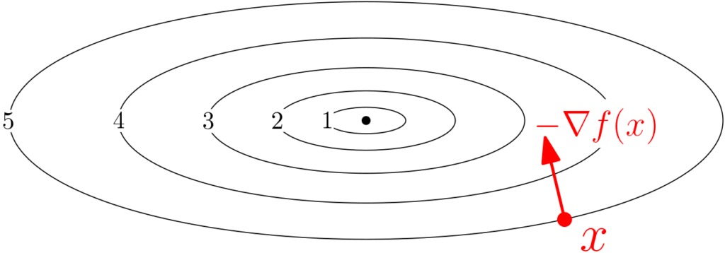
For the \(\ell_2\)-norm, then minimizing \(u^\top \nabla f(x)\) such that \(\|u\|_2 = 1\), leads to $$ \displaystyle u = \ – \frac{\nabla f(x)}{ \| \nabla f(x) \|_2},$$ that is the steepest descent is along the negative gradient (see an illustration below). In this blog post I will only focus on this steepest descent direction.

As as side note, for the \(\ell_1\)-norm, then minimizing \(u^\top \nabla f(x)\) such that \(\|u\|_1 = 1\), leads to $$u \in\ – \arg\max_{ v \in \{-e_1,\, e_1,\, -e_2,\, e_2,\dots,\, -e_d,\, e_d \}} v^\top \nabla f(x),$$ where \(e_i\) is the \(i\)-th canonical basis vector of \(\mathbb{R}^d\). Here the steepest descent is along a coordinate axis (along the positive or negative side), and this leads to various forms of coordinate descent (this will probably be a topic for another post).

Given that the negative gradient leads to the steepest descent direction (for the Euclidean norm), it is natural to use this as a direction for an iterative algorithm, an idea that dates back to Cauchy in 1847 [1] (see the nice summary by Claude Le Maréchal [2]).

From gradient descent to gradient flows

Gradient descent is the most classical iterative algorithm to minimize differentiable functions. It takes the form $$x_{n+1} = x_{n} \, – \gamma \nabla f(x_{n})$$ at iteration \(n\), where \(\gamma > 0 \) is a step-size.

Gradient descent comes in many flavors, steepest, stochastic, pre-conditioned, conjugate, proximal, projected, accelerated, etc. There are lots of papers and books [e.g., 3, 4, 5] analyzing it in various settings.

In this post, to simplify its analysis and setting the stage for later posts, I will present the gradient flow, which is essentially the limit of gradient descent when the step-size \(\gamma\) tends to zero.

More precisely, this is obtained by considering that our iterates \(x_n\) are sampled at each multiple of \(\gamma\), from a function \(X: \mathbb{R}_+ \to \mathbb{R}^d\), as $$x_n = X(n\gamma).$$ We can then use a piecewise affine interpolation to define a function defined on all points. We then have for \(t = n\gamma\), $$X(t + \gamma) = x_{n+1} =x_{n} \, – \gamma \nabla f(x_{n}) = X(t)\, – \gamma \nabla f(X(t)).$$ Dividing by \(\gamma\), we get $$ \frac{1}{\gamma} \big[ X(t + \gamma) \, – X(t) \big] = \, – \nabla f(X(t)).$$

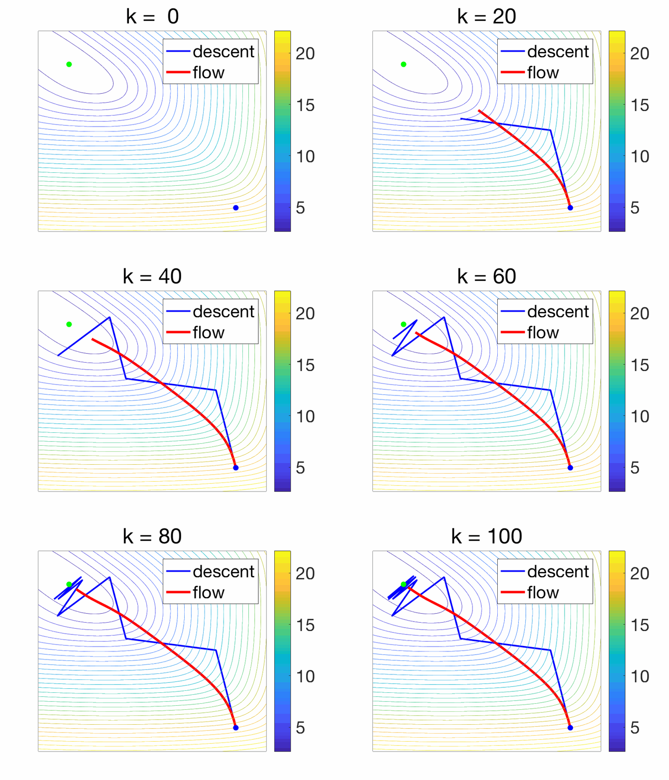
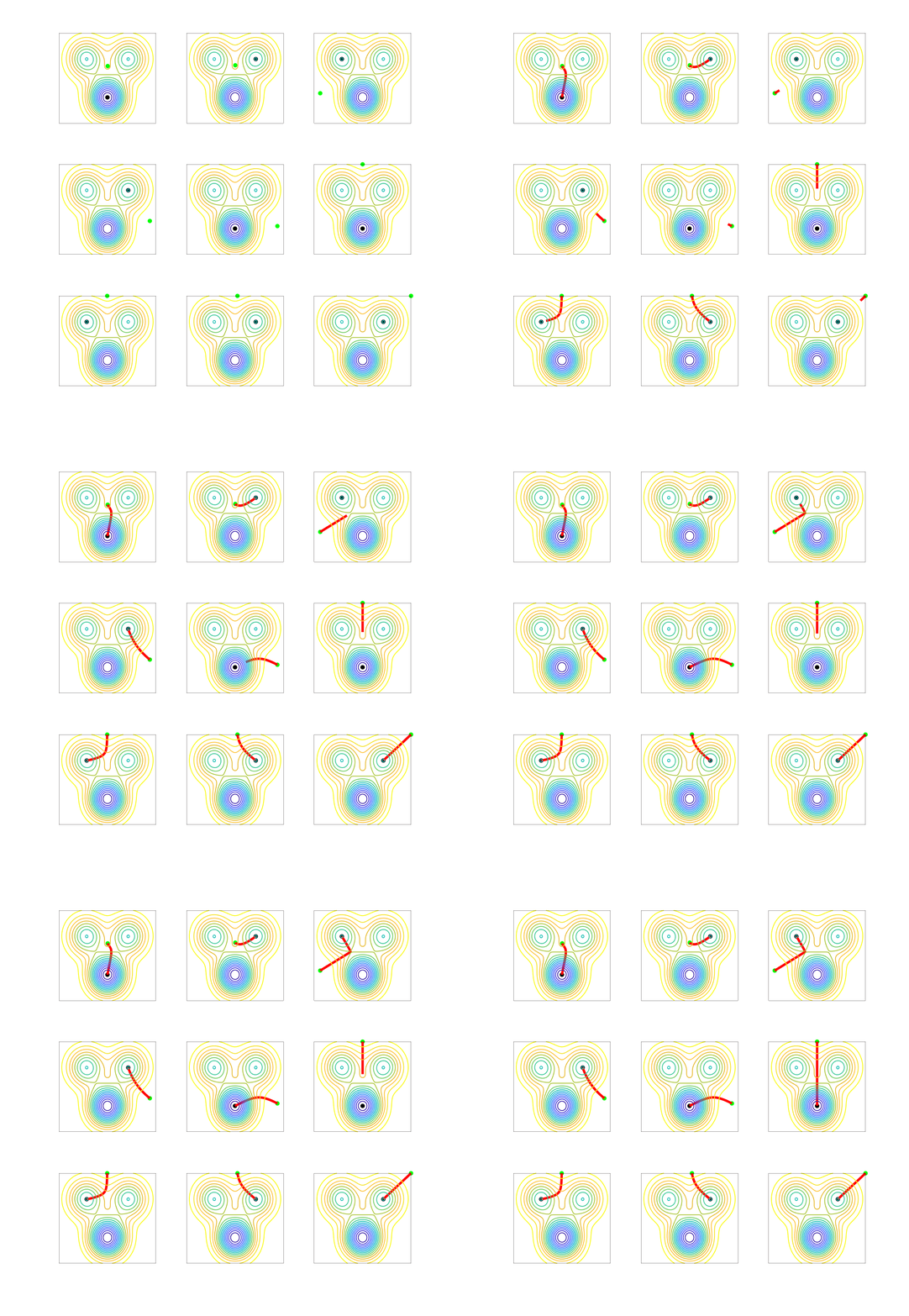
When \(\gamma\) tends to zero (and with simple additional regularity assumptions), the left hand side tends to the derivative of \(X\) at \(t\), and thus the function \(X\) tends to the solution of the following ordinary differential equation $$ \dot{X}(t) = \ – \nabla f (X(t)).$$ See an illustration below.

Studying the gradient flow in lieu of the gradient descent recursions comes with pros and cons.

Simplified analyses. The gradient flow has no step-size, so all the traditional annoying issues regarding the choice of step-size, with line-search, constant, decreasing or with a weird schedule are unnecessary. Moreover, the use of differential calculus makes proving properties really simple (see examples below). We can thus focus on the essence of the algorithm rather than on technicalities.

From (continuous) flow to actual (discrete) algorithms. A flow cannot be run on a computer as it is a continuous-time object. The traditional discretization is the Euler method, that exactly replaces the flow by a piecewise-affine interpolation of the gradient descent iterates, where as shown above, we see \(x_n\) as \(X(n\gamma)\), where \(\gamma\) is the time increment between two samples. Four interesting observations:

• No direct proof transfer : While Euler discretization always provides an algorithm, the generic convergence proofs do not allow to transfer immediately continuous-time proofs to convergence results for the discrete analysis. A key difficulty is to set-up the step-size \(\gamma\). However, the analysis can often be mimicked, i.e., similar Lyapunov functions can be used (see examples below).
• Proximal algorithms : Faced with non-continuous gradient functions, the forward version of Euler discretization \(x_{n+1} = x_{n} – \gamma \nabla f(x_{n})\) can be replaced by the backward version $$x_{n+1} = x_{n} \, – \gamma \nabla f(x_{n+1}),$$ which is only implicit as it can be solved by minimizing $$ f(x) + \frac{1}{2\gamma}\|x-x_{n}\|_2^2,$$ thus leading to the proximal point algorithm. Forward-backward schemes can also be recovered when \(f\) is the sum of a smooth and a non-smooth term.
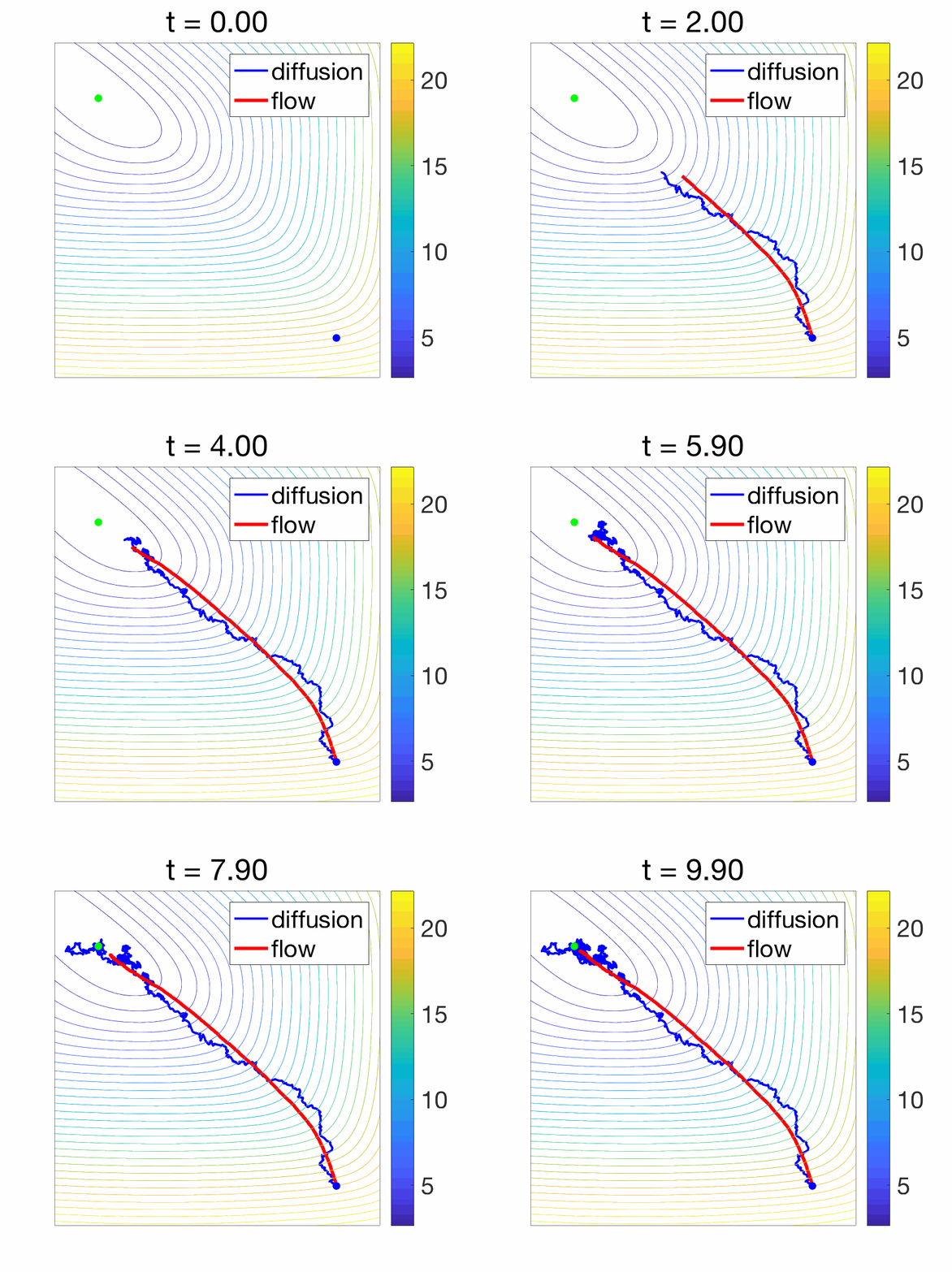
• Stochastic gradient descent : There are two ways to deal with stochastic gradient descent, leading to two very different continuous limits. Adding independent and identically distributed (for simplicity) zero-mean noise \(\varepsilon_n\) to the gradient leads to the recursion $$x_{n+1} = x_{n} – \gamma \big[ \nabla f(x_{n}) + \varepsilon_n\big] = x_{n}\, – \gamma \nabla f(x_{n}) \,- \gamma \varepsilon_n,$$ where the noise is multiplied by the step-size \(\gamma\). Surprisingly, taking the limit when \(\gamma\) tends to zero leads to the deterministic gradient flow equation. A more detailed argument is presented at the end of post, but the main hand-waving reason is that the noise contribution vanishes because it is multiplied by the step-size. Note that this limiting behavior is consistent with a convergence to a minimizer of \(f\).
• Convergence to a Langevin diffusion : When instead the noise is added with magnitude proportional to the square root \(\sqrt{2 \gamma}\) of the step-size (which is asymptotically larger than \(\gamma\)), when \(\gamma\) tends to zero, and if the covariance of the noise is identity, we converge to a diffusion process which is the solution of a stochastic differential equation: $$ dX(t) = \ – \nabla f(X(t)) + \sqrt{2} dB(t),$$ where \(B\) is a standard Brownian motion. Moreover, as \(t\) tends to infinity, \(X(t)\) happens to tend in distribution to a random variable with density proportional to \(\exp( – f(x) )\). See more details at the end of the post and in [6]. The difference in behavior is illustrated below.

Properties of gradient flows

The gradient flow $$ \dot{X}(t) = \ – \nabla f (X(t)) $$ is well-defined for a wide variety of conditions on the function \(f\). The most classical ones are Lipschitz-continuity of the gradient, or semi-convexity [7].

The most obvious property is that the function decreases along the flow; in other words, \(f(X(t))\) is decreasing, which is a simple consequence of $$ \frac{d}{dt} f(X(t)) = \nabla f(X(t))^\top \frac{dX(t)}{dt} =\ – \| \nabla f (X(t) )\|_2^2 \leqslant 0.$$

If \(f\) is bounded from below, then \(f(X(t))\) will always converge (as a non-increasing function which is bounded from below, see here). However, in general, \(X(t)\) may not always converge without any further assumptions, e.g., it may oscillate forever. This is however rare and there are a variety of sufficient conditions for convergence of gradient flows, that date back to Lojasiewicz [8], and are based on “Lojasiewicz inequalities” that state that for \(y\) and \(x\) close enough, \(|f(x) – f(y)|^{1-\theta} \leqslant C \| \nabla f(x)\|\) for some \(C > 0 \) and \(\theta \in (0,1)\). These are satisfied for “sub-analytical functions”, that include most functions one can imagine [9].

Once \(X(t)\) converges to some \(X(\infty) \in \mathbb{R}^d\), assuming \(\nabla f\) is continuous, we must have \(\nabla f(X(\infty))=0\), that is, \(X(\infty)\) is a stationary point of \(f\). Among all stationary points (that can be local minima, local maxima, or saddle-points), the one to which \(X(t)\) converges to depends on \(X(0)\).

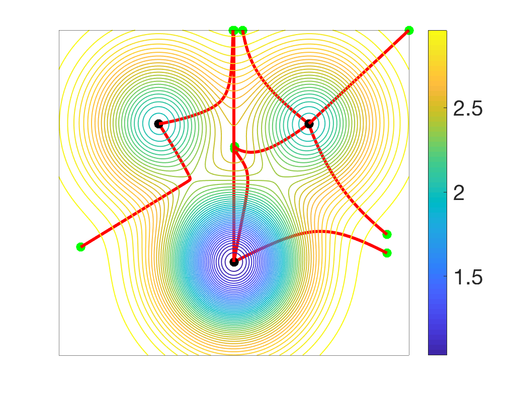
Given any stationary point, one can look at the set of initializations that lead to it. Typically, only local minima are stable, that is, the attraction basins of other stationary points has typically zero Lebesgue measure (see, e.g., [10]). See examples below.

We start with a simple function defined on the two-dimensional plane, with several local minima and saddle-points.

Before moving on, I cannot resist presenting a “real” two-dimensional example that probably all skiers, hikers, and cyclists with some form of mathematical abilities have thought of, the topographic map. Here is an example below:

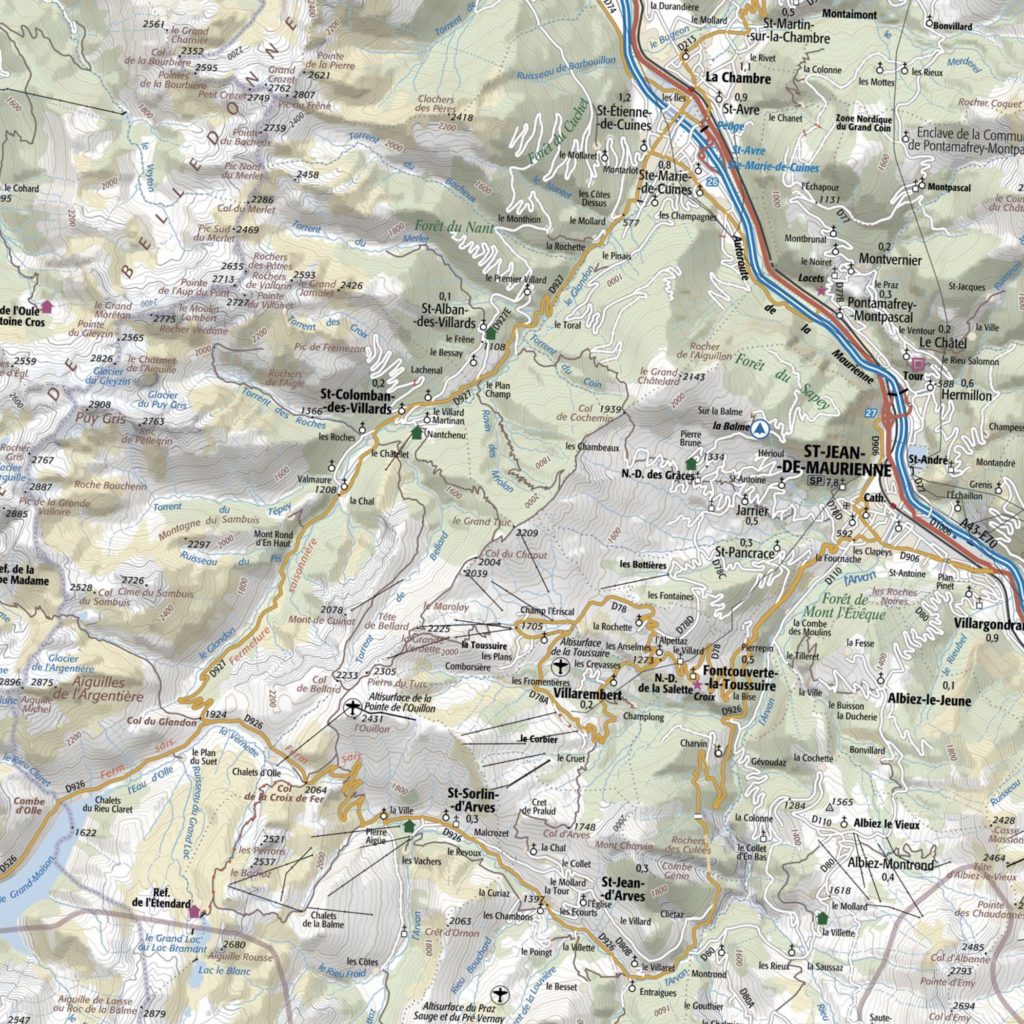
Given the topographic map, how would gradient descent or gradient flow perform? Clearly, this corresponds to a non convex function, but it is quite well-behaved, as following water flows will typically lead to sea level. I chose two starting points famous to cyclists, Col du Glandon and Col de la Croix de Fer, and ran gradient descent with a small step-size (to approximate the gradient flow), without noise (left) and with noise (right), on the topographic map (thanks to Loïc Landrieu for the data extraction).

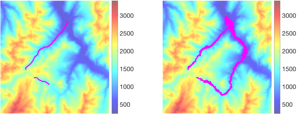
Without noise, the descent from la Croix de Fer ends up getting stuck quickly in a local minimum, while the one from Glandon goes down to the valley, but then is not able to follow the almost flat slope. When noise is added, the two flows go a bit lower, highlighting the benefits of noise to escape local minima.

Gradient flows for optimization and machine learning

There are (at least) two key questions in optimization and machine learning related to gradient flows:

• When can we have global guarantees for convergence? That is, can we make sure that we choose an initialization point well enough to get the the global optimum without knowing where the global optimum is. A key difficulty is that the volume of the attraction basin of the global optimum can be made arbitrarily small, even for infinitely differentiable functions (imagine a function equal to zero everywhere except on a small ball where it is negative).
• How fast can we get there? “there” can be a stationary point or a global optimum. This is an important question as mere convergence in the limit may be arbitrarily slow [11].

An important class of function is convex functions, where everything works out very well. We will study them below. Other functions will be studied in future posts.

Convex functions

We now assume that the function \(f\) is convex and differentiable. Within machine learning, this corresponds to objective functions encountered for supervised learning which are based on empirical risk minimization with a prediction function which is linearly parameterized, such as logistic regression.

There are various definitions of convexity, which are based on global properties (the function is always “below its chords”, or it is always “above its tangents”) or local properties (the Hessian is always positive semi-definite). The one which we need here is to be above its tangents, that is, for any \(x, y \in \mathbb{R}^d\), $$f(x) \geqslant f(y) + \nabla f(y)^\top ( x \, – y).$$ Applying this to any stationary point \(y\) such that \(\nabla f(y)=0\) shows that for all \(x\), \(f(x) \geqslant f(y)\), that is, \(y\) is a global minimizer of \(f\). This is the classical benefit of convexity: no need to worry about local minima.

Another property we will need is the Lojasiewicz inequality, which is in particular satisfied when \(f\) is \(\mu\)-strongly convex (that is, \(f – \frac{\mu}{2} \| \cdot \|_2^2\) is convex): $$ f(x) \ – f(x_\ast) \leqslant \frac{1}{2 \mu} \| \nabla f (x)\|^2$$ for any minimizer \(x_\ast\) of \(f\) and any \(x\). This property allows to go from a bound on the gradient norm to a bound on function values.

We then obtain the convergence rate in one line as follows (see more details in [12]): $$ \frac{d}{dt} \big[ f(X(t))\ – f(x_\ast) \big] =\ \nabla f(X(t))^\top \dot{X}(t) = \ – \| \nabla f(X(t))\|_2^2 \leqslant \ – 2\mu \big[ f(X(t)) \ – f(x_\ast) \big]$$ using the Lojasiewicz inequality above, leading to by simple integration of the derivative of \(\log \big[ f(X(t)) \ – f(x_\ast) \big]\): $$f(X(t)) \ – f(x_\ast) \leqslant \exp( – 2\mu t ) \big[ f(X(0))\ – f(x_\ast) \big], $$ that is, the convergence is exponential and the characteristic time is proportional to \(1/\mu\).

The gradient flow gives the main insight (exponential convergence); and applying the result above to \(t = \gamma n\), we seem to recover the traditional rate proportional to \(\exp( – \gamma \mu n)\); HOWEVER, this is only true asymptotically for \(\gamma\) tending to zero, and proving a result for gradient descent requires extra steps to deal with having a constant step-size. This requires typically \(\gamma \leqslant 1/L\), where \(L\) is the smoothness constant of \(f\), and the simplest proof happens to use the same structure (see [13] and references therein, as well as [14]).

Without strong convexity, we have, using the tangent property at \(X(t)\) and \(x_\ast\): $$ \frac{d}{dt}\big[ \| X(t)\ – x_\ast \|^2 \big] = \ – 2 ( X(t) \ – x_\ast )^\top \nabla f(X(t)) \leqslant \ – 2 \big[ f(X(t)) \ – f(x_\ast) \big],$$ leading to, by integrating from \(0\) to \(t\), and using the monotonicity of \(f(X(t))\): $$ f(X(t)) \ – f(x_\ast) \leqslant \frac{1}{t} \int_0^t \big[ f(X(u)) \ – f(x_\ast) \big] du \leqslant \frac{1}{2t} \| X(0) \ – x_\ast \|^2 \ – \frac{1}{2t} \| X(t) \ – x_\ast \|^2.$$ We recover the usual rates in \(O(1/n)\), with \(t = \gamma n\), with the same caveat as above (the step-size needs to be bounded).

Conclusion

In this blog post, I covered the basic aspects of gradient flows, in particular their relationships with various forms of gradient descent, and their use in obtaining simple convergence justifications. Next months, I will cover extensions of the analyses above, in particular in terms of (1) acceleration for convex functions, where several flows and discretizations are interesting beyond the gradient flow and Euler method [12, 15], and (2) another class of functions which includes non-convex functions as encountered when learning with neural networks [16].

References

[1] Augustin Louis Cauchy. Méthode générale pour la résolution des systèmes d’équations simultanées. Compte Rendu à l’Académie des Sciences, 25:536–538, 1847.
[2] Claude Lemaréchal. Cauchy and the Gradient Method. Documenta Mathematica, Extra Volume: Optimization Stories, 251–254, 2012.
[3] Yurii Nesterov. Introductory lectures on convex optimization: A basic course (Vol. 87). Springer Science & Business Media, 2013.
[4] Dimitri P. Bertsekas, Nonlinear programming. Athena Scientific, 1999.
[5] Jorge Nocedal and Stephen Wright. Numerical optimization. Springer Science & Business Media, 2006.
[6] Arnak S. Dalalyan. Theoretical guarantees for approximate sampling from smooth and log‐concave densities. Journal of the Royal Statistical Society: Series B (Statistical Methodology), 79(3), 651-676, 2017.
[7] Filippo Santambrogio. {Euclidean, metric, and Wasserstein} gradient flows: an overview. Bulletin of Mathematical Sciences, 7(1), 87-154, 2017.
[8] Stanislaw Lojasiewicz. Sur les trajectoires du gradient d’une fonction analytique. Seminari di Geometria, 1983:115–117, 1982.
[9] Jérôme Bolte, Aris Daniilidis, and Adrian Lewis. A nonsmooth Morse–Sard theorem for subanalytic functions. Journal of Mathematical Analysis and Applications, 321(2):729–740, 2006.
[10] Jason D. Lee, Max Simchowitz, Michael I. Jordan, Benjamin Recht. Gradient descent only converges to minimizers. Conference on learning theory, 1246-1257, 2016.
[11] Simon S. Du, Chi Jin, Jason D. Lee, Michael I. Jordan, Barnabas Poczos, Aarti Singh. Gradient descent can take exponential time to escape saddle points. Advances in neural information processing systems, 1067-1077, 2017.
[12] Damien Scieur, Vincent Roulet, Francis Bach, Alexandre d’Aspremont,. Integration methods and optimization algorithms. Advances in Neural Information Processing Systems, 1109-1118, 2017.
[13] Hamed Karimi, Julie Nutini, Mark Schmidt. Linear convergence of gradient and proximal-gradient methods under the Polyak-Lojasiewicz condition. Joint European Conference on Machine Learning and Knowledge Discovery in Databases, 795-811, 2016.
[14] Boris T. Polyak. Gradient methods for minimizing functionals. Zh. Vychisl. Mat. Mat. Fiz., 3(4):643–653, 1963.
[15] Weijie Su, Stephen Boyd, Emmanuel J. Candès. A differential equation for modeling Nesterov’s accelerated gradient method: theory and insights. Journal of Machine Learning Research, 17(1), 5312-5354, 2017.
[16] Lénaïc Chizat, Francis Bach. On the global convergence of gradient descent for over-parameterized models using optimal transport. Advances in Neural Information Processing Systems, 3036-3046, 2018.

Limits of stochastic gradient descent for vanishing step-sizes

Convergence to gradient flow. We consider fixed times \(t = n \gamma \) and \(s = m \gamma\), and we let \(\gamma\) tend to zero, with thus \(m\) and \(n\) tending to infinity. Starting from the recursion $$x_{n+1} = x_{n}\, – \gamma \nabla f(x_{n})\ – \gamma \varepsilon_n,$$ we get the following by applying it \(m\) times: $$X(t+s) \ – X(t) = x_{n+m}-x_n = \ – \gamma \sum_{k=0}^{m-1} \nabla f\Big(X\Big(t+\frac{sk}{m}\Big)\Big)\ – \gamma \sum_{k=0}^{m-1} \varepsilon_{k+n}.$$ The term \(\displaystyle \gamma \sum_{k=0}^{m-1} \nabla f\Big(X\Big(t+\frac{sk}{m}\Big)\Big)\) converges to \(\displaystyle \int_{t}^{t+s}\!\!\! \nabla f(X(u)) du\), while the term \(\gamma \sum_{k=0}^{m-1} \varepsilon_{k+n}\) has zero expectation and variance equal to \(\gamma^2 m = \gamma s \) times the variance of each \(\varepsilon_{k+n}\), and thus it tends to zero (since \(\gamma\) tends to zero). Thus, in the limit, $$X(t+s)\ – X(t) = \ – \int_{t}^{t+s} \!\!\! \nabla f(X(u)) du,$$ which is equivalent to the gradient flow equation.

Convergence to diffusion. We consider the recursion $$x_{n+1} = x_{n}\, – \gamma \nabla f(x_{n}) + \sqrt{2\gamma} \varepsilon_n.$$ With the same argument as above, we now get $$X(t+s) \ – X(t) = x_{n+m}-x_n =\ – \gamma \sum_{k=0}^{m-1} \nabla f\Big(X\Big(t+\frac{sk}{m}\Big)\Big)\ – \sqrt{2\gamma} \sum_{k=0}^{m-1} \varepsilon_{k+n}.$$ Now the second term has zero mean but a variance proportional to \(2s\) (which does not go to zero when \(\gamma\) goes to zero). We can then use when \(m\) tends to infinity the limit of the sum of independent variables as a Wiener process, to get $$X(t+s)\ – X(t) =\ – \int_{t}^{t+s} \!\!\! \nabla f(X(u)) du + \sqrt{2} \big[ B(t+s)-B(t) \big].$$ The limiting distribution of \(X(t)\) happens to be the so-called Gibbs distribution, with density \(\exp(-f(x))\) (the factor of \(\sqrt{2}\) was added to avoid an extra constant factor in the Gibbs distribution). More on this in a future post.