Rethinking SGD’s noise – II: Implicit Bias

In the previous post, we showed (or at least tried to!) how the inherent noise of the stochastic gradient descent algorithm (SGD), in the context of modern overparametrised architectures, is structured and carries two important features: (i) it vanishes for interpolating solutions and (ii) it belongs to a low-dimensional manifold spanned by the gradients.

Building on this, we will go deeper and try to understand how SGD’s noise affects the training trajectories. Indeed there have been several empirical hints [1, 25] which suggest that when it comes to training a neural network for various real-world prediction tasks, the structured noise in SGD is beneficial for generalisation in comparison to full batch gradient descent (GD). This intriguing observation moves beyond the classical stochastic optimisation viewpoint where the sampling in SGD is simply a trick to lower the gradient computation complexity. In this blogpost we will explore the following question.

How can we explain that the inherent noise in SGD drives the dynamics towards a solution which is differently structured than that of GD?

Keep in mind that we do not pretend to treat these questions in the context of complex neural networks, but we will rather focus on simpler architectures which are already enlightening. Starting from a simple convex case before moving to more complex architectures, there is a long but exciting journey ahead! Yet, first comes first and let us start by properly introducing the framework.

The need to understand the implicit bias

The current architectures which are used to solve supervised learning tasks are known to be largely overparametrised. This means that the parametric function space \(\mathcal{F} = \{x \mapsto f_\theta(x),\ \theta \in \mathbb{R}^p \}\) is described by some high-dimensional parameter \(\theta \in \mathbb{R}^p\) where \(p\) is much larger than the number \(n\) of training samples \((x_i, y_i)_{1 \leqslant i \leqslant n} \in \mathbb{R}^d \times \mathbb{R}\). Two canonical examples of such classes are:

An important consequence of having overparametrised models is that the space of all the parameters which perfectly interpolate the training set, i.e., the space \(\mathcal{I}_\mathcal{F} := \{\theta^* \in \mathbb{R}^p \ \mathrm{s.t.}\ f_{\theta^*}(x_i) = y_i\}\), is (under a few assumptions) a manifold of dimension \(p \, – n \gg 1\) [2]. Hence, if one wants to optimise the empirical risk $$\mathcal{R}(\theta) = \frac{1}{2n} \sum_{i=1}^n (f_\theta(x_i) \,- y_i)^2, $$ then any element \(\theta^*\) of \(\mathcal{I}_\mathcal{F}\) is a global minimiser of \(\mathcal{R}\) with \(\mathcal{R}(\theta^*) = 0\). Keep in mind that throughout this blogpost, \(\mathcal{R}\) will always correspond to the “train loss” and that we will never consider the “test loss”. Now assume that we have an algorithm that successfully converges to a global minimum of \(\mathcal{R}\): it is a priori unclear which predictive function \(f_{\theta^*} \in \mathcal{F}\) we have retrieved amongst the infinitude of interpolating functions. This is annoying since we know that highly parametrised neural networks can easily fit random noise, therefore our recovered \(f_{\theta^*}\) could be arbitrarily badly behaved and perform very poorly on unseen data. This is often refered to as “overfitting”.
However, it has been empirically noticed again and again that the classical training procedures used in the ML community (GD, SGD, momentum, etc.) lead to the recovery of solutions which perfectly fit the training set and generalise well [3]! This is highly non-trivial and means that the algorithm which is used for the training must be responsible of this success by converging towards a well-behaved solution (see Figure 1). A natural and central question is therefore:

Towards which interpolator did our algorithm lead us?

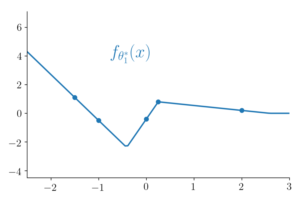
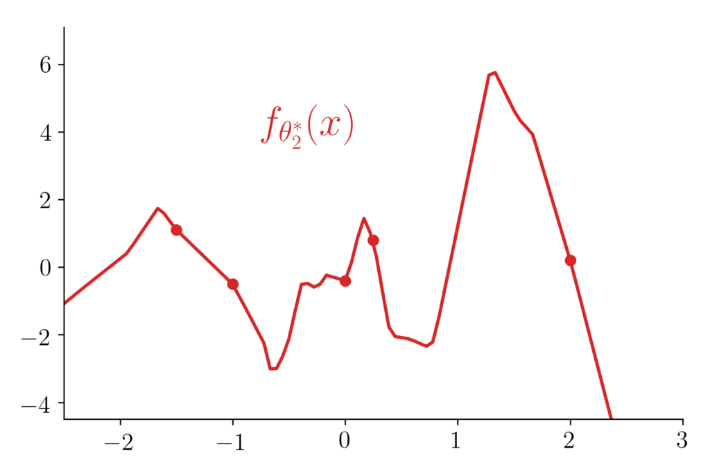
Figure 1: Different interpolators behave and generalise differently. For the anecdote, the two plotted functions are 2-layer ReLU-networks which have both been trained with gradient descent but with 2 very different initialisations. Puzzling right? But let us keep this story for another time [23].

This “algorithmic interpolator selection” phenomenon is commonly named algorithmic regularisation or also implicit bias due to the fact that no explicit regularisation which constrains the set of minimisers is added to the loss during training [3, 4, 5, 6].

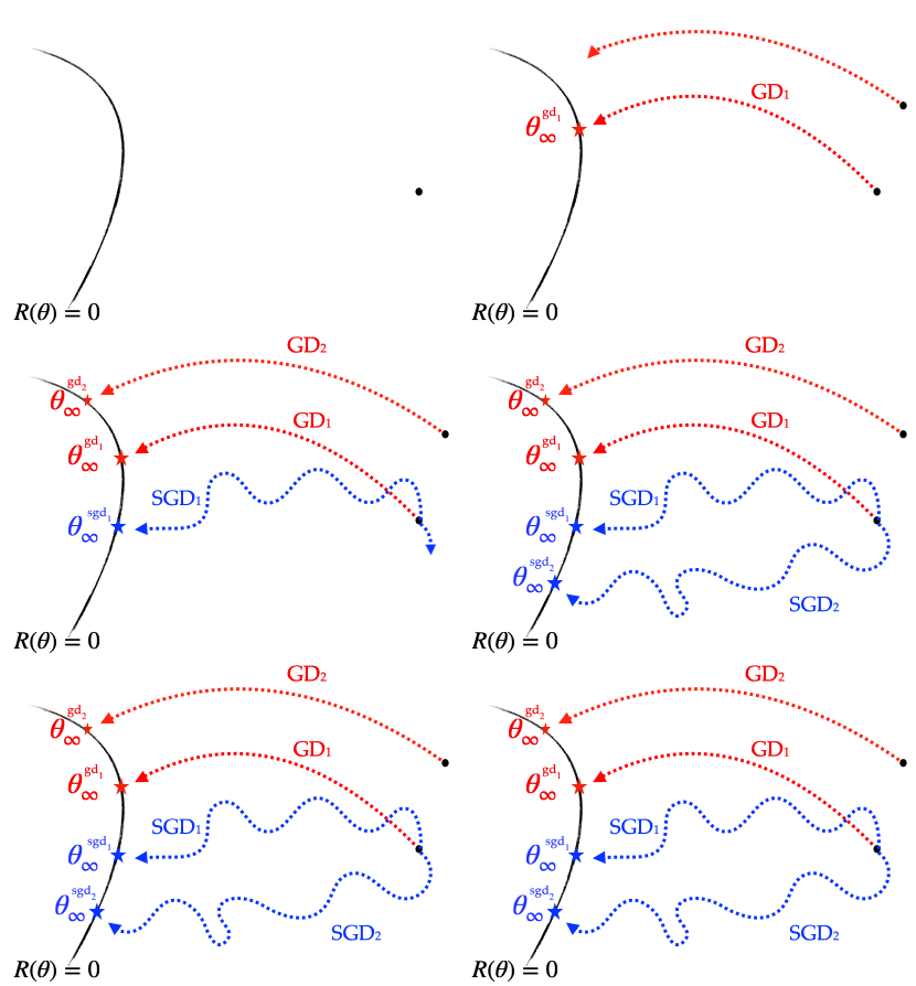
Figure 2: Different algorithms have different implicit biases: they converge to distinct global solutions. Here are schematically displayed two gradient descent trajectories with different initialisations as well as two stochastic gradient descent trajectories with the same initialisation but different random seeds.

A warm-up: the least-squares setting

To make things clear and exhibit how an algorithmic regularisation can be characterised, we will start with Francis’ favorite machine learning friend, the least squares setting!

Let us consider the linearly parametrised family of linear predictors \(x \in \mathbb{R}^d \mapsto \langle \beta, x \rangle\), for \(\beta \in \mathbb{R}^d\). Let \((x_i, y_i)_{1 \leqslant i \leqslant n}\) be the \(n\) input/output samples we have at hand, and let’s encapsulate them in the vector \(y \in \mathbb{R}^n\) and the design matrix \(X \in \mathbb{R}^{n \times d}\) whose \(i^{th}\) line is the vector \(x_i \in \mathbb{R}^d\). The empirical risk \(\beta \mapsto \mathcal{R}(\beta)\) is then a simple quadratic and convex function (note here that we use \(\beta := \theta\) for notation coherence with the future sections), and hence [7] any gradient method with proper step size will converge towards a global minimum \(\beta^*\) with \(X \beta^* = y\), i.e., a point which perfectly fits the dataset.

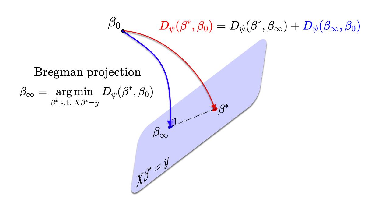
Let us denote \(\beta_\infty^{\text{gd}}\) and \(\beta_\infty^{\text{sgd}}\) the two limiting points of the GD and SGD dynamics. Remarkably, the linearity offers a nice geometric argument [8] that allows to characterise exactly \(\beta_\infty^{\text{gd}}\) as well as \(\beta_\infty^{\text{sgd}}\). Indeed, notice that for all \(\beta \in \mathbb{R}^d\), the full gradient writes \(\nabla \mathcal{R}(\beta) = \frac{1}{n} X^\top (X \beta\, – y) \in \text{span}\{x_1, \dots, x_n\}\), and a stochastic gradient also writes \(\nabla \mathcal{R}_{i_t}(\beta) = x_{i_t} (\langle x_{i_t}, \beta \rangle\, – y_{i_t}) \in \text{span}\{x_1, \dots, x_n\}\) with \(i_t\) sampled uniformly in \(\{1, \dots, n\}\). Therefore, all the GD and SGD iterates belong to the affine space \(\beta_0 + \text{span}\{x_1, \dots, x_n\}\), where \(\beta_0\) is the initialisation. Hence, assuming that the step size is not too big and that the iterates converge, the same will hold for their limiting points: $$\beta_\infty^{\text{gd}},\ \beta_\infty^{\text{sgd}} \in \beta_0 \,+\, \text{span}\{x_1, \dots, x_n\}.$$ On the other hand, the manifold of interpolators \(\mathcal{I}_{\mathcal{F}} = \{\beta^* \in \mathbb{R}^d\ \mathrm{s.t.} \ \langle \beta^*, x_i \rangle = y_i, \forall i\}\) is the affine space \(\beta^* + \mathrm{span}\{x_1, \dots, x_n\}^\perp \) where \(\beta^*\) is any interpolator in \(\mathcal{I}_{\mathcal{F}}\). Therefore we have that \(\beta_\infty^{\text{gd}} – \beta_0 \perp \beta_\infty^{\text{gd}} – \beta^*,\) and the same holds for \(\beta_\infty^{\text{sgd}}\). This means, by Pythagoras’ theorem that \(\Vert \beta^* – \beta_0 \Vert^2 = \Vert \beta^* – \beta_\infty \Vert^2 + \Vert \beta_\infty – \beta_0 \Vert^2\) and $$\beta_\infty^{\text{gd}} = \beta_\infty^{\text{sgd}} = \underset{\beta^* \ \mathrm{s.t.} \ X \beta^* = y}{\arg \min}\ \Vert \beta^* \,- \beta_0\Vert_2^2,$$ which also means that \(\beta_\infty^{\text{gd}} = \beta_\infty^{\text{sgd}} = \pi_{\mathcal{I}}(\beta_0)\), where \(\pi_{\mathcal{I}}\) is the orthogonal projection on \(\mathcal{I}_\mathcal{F}\). Here is a geometrical sketch of what is going on:

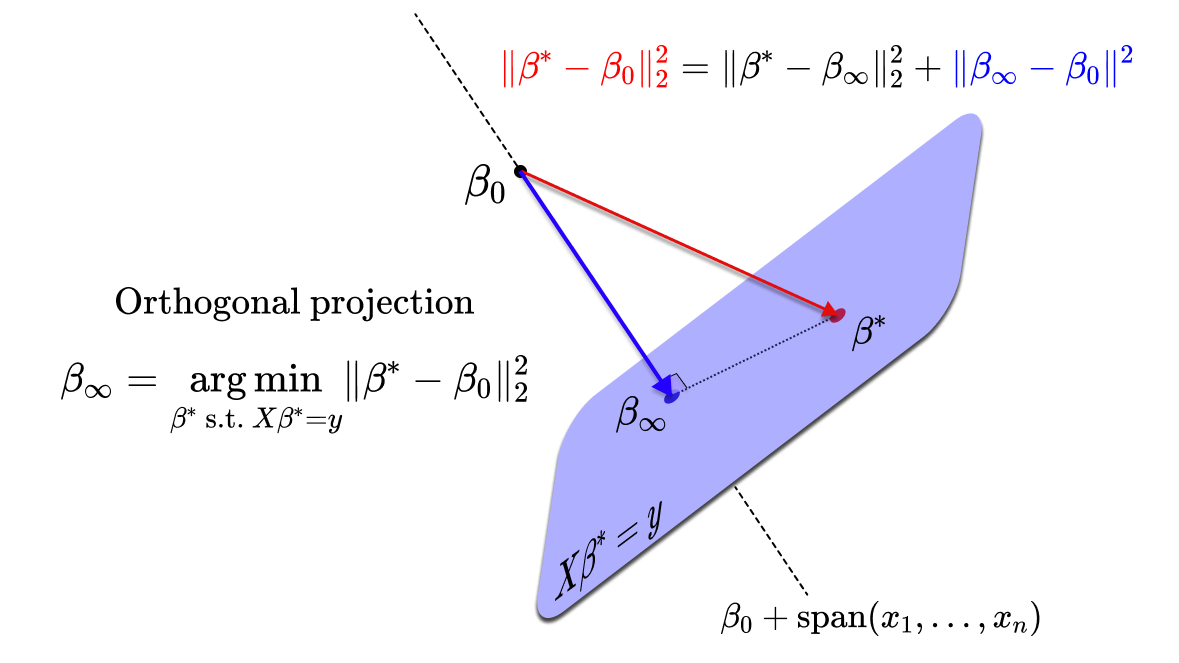
This implicit regularisation problem uniquely characterises the solutions retrieved by GD and SGD. Note that in this linear setting, the stochasticity of SGD does not change the limiting point of the dynamics: even though SGD is stochastic, its limiting point is deterministic and exactly the same as for gradient descent (for the same initialisation of course).

Moving on to a simple but rich neural architecture

Considering the implicit regularisation of GD and SGD on linearly parametrised models is a great starting point to understand the notion. However as we have just seen, in this case, they both have the same associated implicit regularisation problem. This is a bit disappointing since we know that this is not the case for more complex architectures: the noise inherent to SGD seems to significantly improve its performance on unseen data [1, 25]. To take a first step towards understanding this for complex architectures, we will let the linear parametrisation aside, and consider a toy (nonetheless very rich!) “neural network” that has received a lot of attention lately [9, 10, 11] (to cite a few).

A toy network: the \(2\)-layer linear diagonal network. Let us introduce our toy neural network, which has (so far!) absolutely no practical relevance, but has the merit of unveiling many training characteristics which occur in much more complex architectures. This network is called a \(2\)-layer linear diagonal network and is illustrated below (right plot).

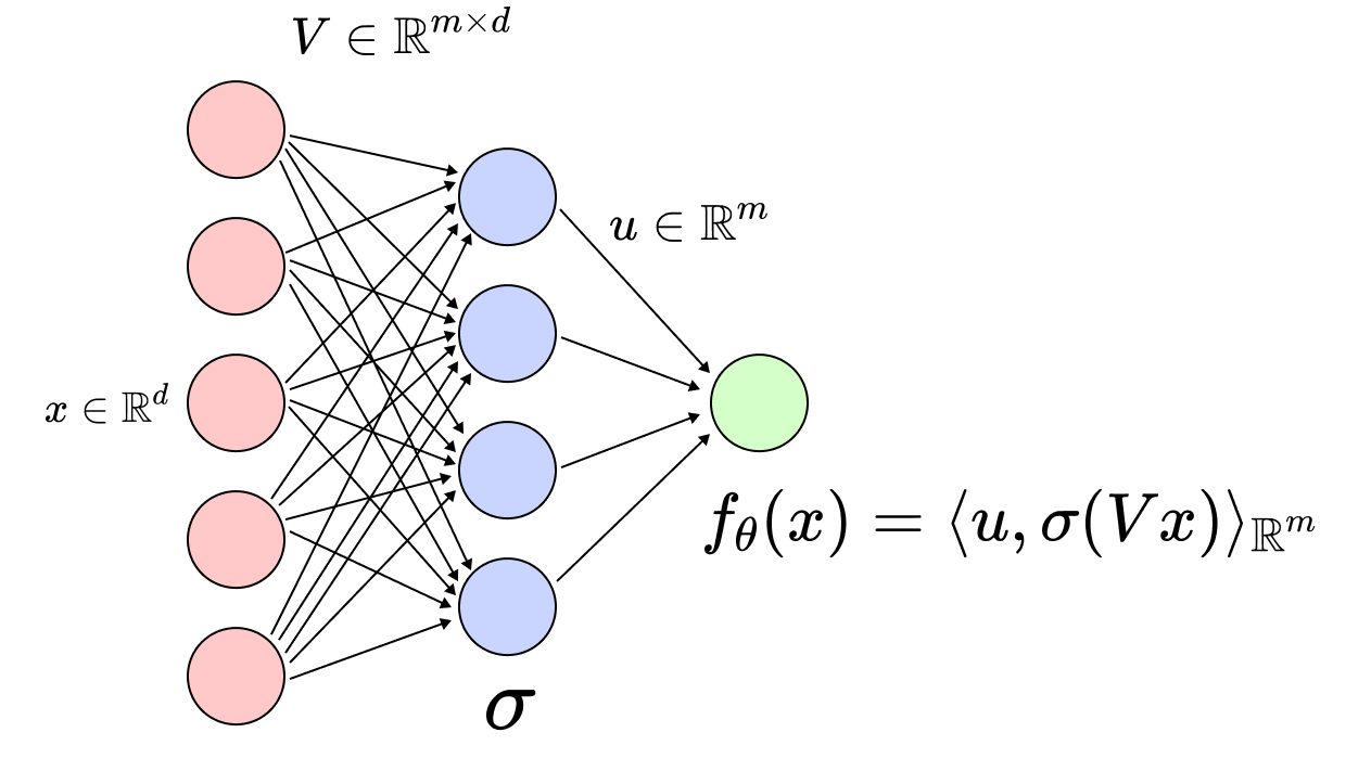
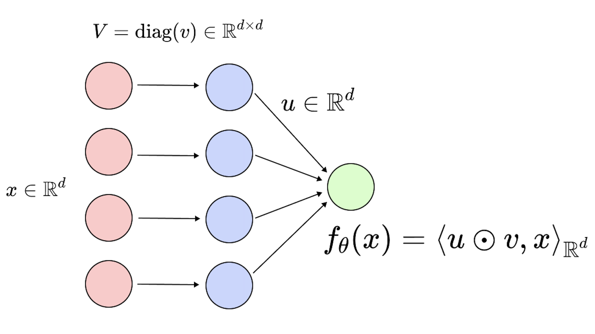
Figure 3: Left: fully connected 2-layer neural network \(f_\theta(x) = \langle u, \sigma(V x) \rangle_{\mathbb{R}^m} \), and \(\theta = (u, V) \in \mathbb{R}^m \times \mathbb{R}^{m\times d}\). Right: linear diagonal network \(f_\theta(x) = \langle u, v \odot x \rangle\), and \(\theta = (u, v) \in \mathbb{R}^{2d}\).

As you can notice in the illustration, each neuron from the first layer is only connected to one input entry, this means that the associated weight matrix has a diagonal structure (hence the name). The first layer, \(v \in \mathbb{R}^d\), can be considered as a vector instead of a diagonal matrix, and the second layer is denoted by \(u \in \mathbb{R}^d\). As the name suggests, we do not add any non-linear activation between the two layers. Equipped with these notations, the prediction function associated to this architecture writes \(f_\theta(x) = \langle u \odot v, x \rangle\), with \(\theta = (u, v) \in \mathbb{R}^{2d}\), where \(\odot\) is the element-wise product in \(\mathbb{R}^d\).

As you can notice, \(f_\theta\) is linear in \(x\) and we have simply reparametrised our linear predictor from the previous section as \(\beta := u \odot v \in \mathbb{R}^d\). This can seem disappointing since the class of prediction functions is exactly the same as before. But as we will see, this reparametrisation highly changes the training dynamics as well as the algorithmic regularisation of gradient methods. For a start, note that the empirical risk is no longer convex in \(\theta = (u, v)\)! $$ \mathcal{R}(\theta) = \frac{1}{2 n} \sum_{i = 1}^n (y_i \,- \langle u \odot v , \ x_i\rangle )^2 = \frac{1}{2 n} \Vert y\, – X (u \odot v) \Vert_2^2,$$ where we recall that \(y \in \mathbb{R}^n\) is the observation vector and \(X \in \mathbb{R}^{n \times d}\) is the feature matrix. Because of non-convexity, we have a priori no global convergence guarantees for standard algorithms such as gradient descent or even gradient flow.

Gradient flow training dynamics. We follow [10] and consider the continuous time version of gradient descent: gradient flow. Indeed as pointed out in a previous blog post, the continuous counterpart very often leads to much simpler and clearer computations (understand: we don’t know how to do the analysis in discrete time). For simplicity, we will assume that we initialise the weights as \(u_{t = 0} = \alpha \mathbf{1} \in \mathbb{R}^d\) and \(v_{t = 0} = \mathbf{0} \in \mathbb{R}^d\), where \(\alpha > 0 \) is the initialisation scale, \(\mathbf{1}\) the vector of ones and \(\mathbf{0}\) the vector of zeros. Keep this \(\alpha\) parameter in mind as we will see later that it plays a decisive role! Also note that for such an initialisation, we have that \(\beta_{t = 0} = u_{t = 0} \odot v_{t=0} = 0\) whatever \(\alpha\). The gradient flow writes: $$ \dot u_t =\, – \frac{1}{n} [X^{\top} r_t] \odot v_t \quad \mathrm{and} \quad \dot v_t =\, – \frac{1}{n} [X^{\top} r_t] \odot u_t, $$ where \(r_t := X (u_t \odot v_t)\, – y = X \beta_t\, – y \in \mathbb{R}^n\) is the residual vector at time \(t\) with \(\beta_t := u_t \odot v_t\). Since our prediction function \(f_{\theta_t}(x) = \langle x, u_t \odot v_t \rangle\) depends in fine only on \(\beta_t\), a natural question to ask is what type of flow do the predictors \((\beta_t)_{t \geq 0}\) follow?

Surprisingly, it can be shown [10] (detailed calculations in the Appendix) that \((\beta_t)_{t \geq 0}\) follows a mirror flow on the convex loss \(\beta \mapsto \mathcal{R}(\beta) = \Vert X \beta\, – y \Vert_2^2 / (2n)\) and with the hyperbolic entropy as a potential. We denote by \(\phi_\alpha: \mathbb{R}^d \to \mathbb{R}\) this potential as it depends on the initialisation scale (its exact expression is uninformative but can be found in the Appendix). In concise math, this means that for all \(t>0\), $$\frac{\mathrm{d}}{\mathrm{d} t} \nabla \phi_\alpha(\beta_t) =\, – \nabla_\beta \mathcal{R}(\beta_t).$$ For those who are not familiar with the mirror descent algorithm [11, 12], you can think of it as a generalisation of gradient descent but where the distance is not the classical \(\ell_2\)-distance but a Bregman divergence.

Let us provide the reader a quick recap to keep the ideas clear: the non-convex gradient flow on the neurons \((u_t, v_t)_t \in \mathbb{R}^{2d}\) with initialisation scale \(\alpha\) corresponds to a convex mirror flow on the predictors \(\beta_t = u_t \odot v_t\in \mathbb{R}^d\) with potential \(\phi_\alpha\).

Mirror flow: so what? It turns out that now that we have written the predictor dynamics as a mirror flow, everything will become much simpler. Indeed we have passed from a gradient flow on a non-convex loss to a mirror flow on a convex loss. We can therefore leverage many existing results from the literature. Let us forget our particular \(\phi_\alpha\) for a moment and consider a general mirror descent framework with a strictly convex potential \(\psi : \mathbb{R}^d \to \mathbb{R}\).

Convergence: the loss \(\mathcal{R}\) being convex in \(\beta\), we can easily obtain convergence guarantees of the loss using classical results from the literature [12]. And with a bit more work, we can also show that the iterates must converge to an interpolator which we denote \(\beta_\infty\): \(\beta_t \underset{t \to \infty}{\to} \beta_\infty\).

Implicit bias: it remains to characterise \(\beta_\infty\) amongst all the possible interpolators. It turns out that, similarly to the linear framework in the previous section, we can easily describe the algorithmic bias of mirror descent (and mirror flow) [13, 14]. Since \(\mathrm{d} \nabla \psi (\beta_t) =- \frac{1}{n} X^\top (X \beta_t\, – y) \mathrm{d} t\), we have that for all \(t>0\), the “dual” iterates lie in a fix affine space: \(\nabla \psi(\beta_t) \in \nabla \psi(\beta_0) + \mathrm{span}(x_1, \dots, x_n)\). Hence the same holds at the limit. Now a bit of geometry: the law of cosines adapted to the Bregman divergence gives for any interpolator \(\beta^*\): $$D_\psi(\beta^*, \beta_0) = D_\psi(\beta^*, \beta_\infty) + D_\psi(\beta_\infty, \beta_0) + \langle \nabla \psi(\beta_\infty)\, – \nabla \psi(\beta_0), \beta^* – \beta_\infty \rangle. $$ As \(\nabla \psi(\beta_\infty)\, – \nabla \psi(\beta_0) \in \mathrm{span}(x_1, \dots, x_n)\) and \(\beta^* – \beta_\infty \perp \mathrm{span}(x_1, \dots, x_n)\) (because \(X(\beta^* – \beta_\infty) = 0\)) we immediately get that \(D_\psi(\beta^*, \beta_0) = D_\psi(\beta^*, \beta_\infty,) + D_\psi(\beta_\infty, \beta_0) \): this corresponds to Pythagoras’ theorem but for the Bregman divergence. From here, using the strict non negativity of the Bregman divergence (due to the strictly convex \(\psi\)) we obtain $$ \beta_\infty = \underset{ \beta^* \ \mathrm{s.t.} \ \ X \beta^* = y}{ \arg \min} \ D_\psi(\beta^*, \beta_0).$$ Similarly to the linear case, this means that the recovered interpolator \(\beta_\infty\) is the closest to the initialisation with respect to the Bregman divergence (i.e., the Bregman projection on the interpolation space).

Back on topic. Now that we understand the convergence and the algorithmic bias of mirror flow, we can simply apply these results to our setting with \(\psi = \phi_\alpha\). We get that the iterates \((\beta_t)_{t \geq 0}\) converge to some \(\beta_\infty^\alpha\) which highly depends on the neural activation scale \(\alpha\) and satisfies: $$\beta^\alpha_\infty = \underset{ \beta \ \mathrm{s.t.} \ X \beta = y}{ \text{argmin}}\ \phi_\alpha(\beta),$$ because \(\beta_{t = 0} = 0\) and \(D_{\phi_\alpha}(\beta, 0) = \phi_\alpha(\beta)\) for our particular \(\phi_\alpha\). This is exactly the result of Woodworth et al. [10]: let us put this result in perspective as perfectly done in the mentioned paper.

Role of the initialisation. The initialisation scale \(\alpha\) has a huge impact on the recovered solution as it changes the behavior of \(\phi_\alpha\). We can distinguish two major behaviours:

Kernel/lazy regime: for large initialisations, we can show that \(\phi_\alpha\) is close to the \(\ell_2\)-norm, which means that we recover the solution with the minimum \(\ell_2\)-norm. This is consistent with the lazy regime [15]: using a large initialisation, the weights \((u_t, v_t)\) will relatively barely move and we can perform a Taylor expansion around the initialisation. In this case we are back to the linear setting and the neurons will converge towards the closest interpolator (in \(\ell_2\)-distance), this also corresponds to the closest interpolator in predictor space.

Rich regime: for small initialisations the Taylor expansion does not hold anymore, and the training dynamics are more complex. We can show that \(\phi_\alpha \underset{\alpha \to 0}{\sim} \Vert \cdot \Vert_1\), and the recovered solution will therefore enjoy some sparsity guarantees which can be beneficial in terms of generalisation in many settings. A natural question is why not simply take \(\alpha = 0\), i.e., initialise the neurons exactly at \(0\). The problem here is that \(0\) is a saddle point of the loss \(\mathcal{R}(u, v)\): \(\nabla \mathcal{R}(u = 0, v = 0) = 0\). Hence the neurons will not move if exactly initialised at the origin. In the same logic, the smaller we take the initialisation, the longer it takes the neurons to escape the \(0\) saddle, and hence the longer the training time for the iterates to converge to an interpolator. There is therefore an implicit bias/optimisation trade off.

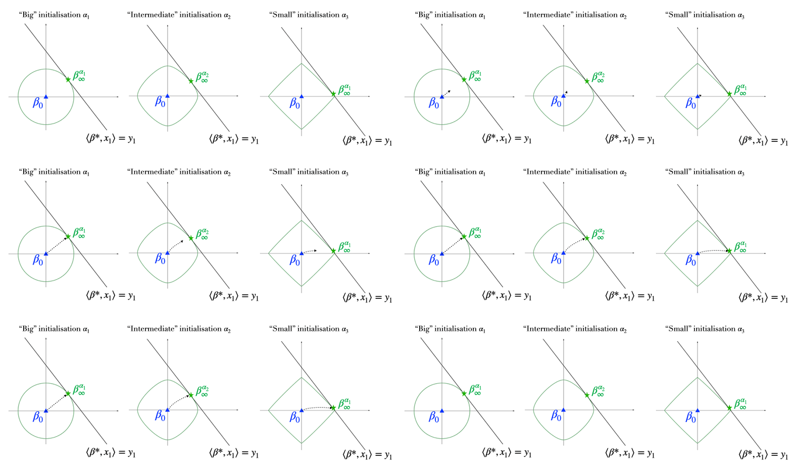
Figure 4: Role of the initialisation scale \(\alpha\) on the structure of \(\beta_\infty^\alpha\): the smaller the neural activation scale \(\alpha\), the lower the \(\ell_1\)-norm of the recovered interpolator but the slower the dynamics. The arrows correspond to the trajectories of the \(\phi_\alpha\)-mirror flow \((\beta_t)_t\) and the balls correspond to level lines of the function \(\phi_\alpha\) for three values of \(\alpha\).

The role of noise

In the previous section, we saw that the initialisation scale is a crucial hyper-parameter which can drastically change the structure of the retrieved interpolator. We will now focus on the role of the noise of SGD. Surprisingly, even though it has been empirically shown to play an important role in the generalisation performances of neural nets, its effect seems much more difficult to understand [16]. In recent years, an interesting approach has been to argue that the invariant distribution of the SGD dynamics concentrates in regions where the loss landscape is “flat” [17]. However as we saw in the previous blogpost, because of the high overparametrisation of modern architectures, the stochastic noise vanishes at global optima. Hence (and as observed in practice), the iterates can converge even with a fixed step size, and this contradicts the invariant distribution viewpoint. In this blog post we take a different approach: in the framework of our toy diagonal network, we will indeed see that iterates converge (with high probability) towards a global optimum and we will even be able to characterise the structure of this solution.

Let us first motivate our approach by taking a look at the figure below: when considering a sparse regression problem with our \(u \odot v\) parametrisation, the solution recovered by SGD is much closer to the minimum \(\ell_1\) interpolator, \(\beta^*_{\ell_1} := \text{argmin}_{\beta, \ X \beta = y} \Vert \beta \Vert_1\), than the one recovered by GD!

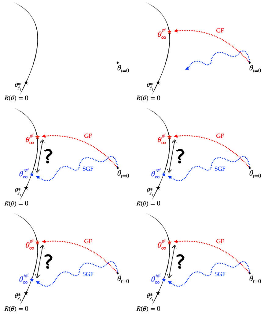
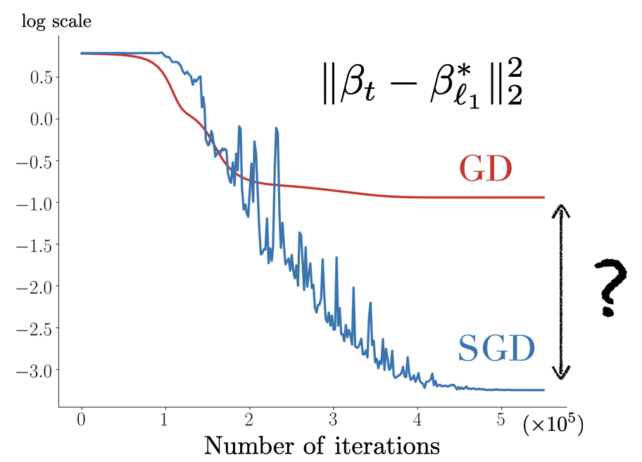
Figure 5: Left (Drawing). parameter space \(\theta = (u, v) \in \mathbb{R}^{2 d}\): for diagonal linear networks, the solutions recovered by SGD and GD differ. Right. Sparse regression using the diagonal network with \(n = 40\), \(d = 100\), \(\Vert \beta^*_{\ell_1} \Vert_0 = 5\), \(x_i \sim \mathcal{N}(0, I)\), \(y_i = \langle x_i, \beta^*_{\ell_1} \rangle \). SGD converges towards a solution which is closer than GD to the minimum \(\ell_1\) norm solution by more than an order of magnitude.

Now that we have a clear experimental setup where GD and SGD have significant different implicit biases, let us try to understand this phenomenon. We follow the line of our work with Nicolas Flammarion [18].

From discrete to continuous. As for GD, we do not know how to conduct the analysis in discrete time and we will therefore switch to the painless continuous paradigm. As seen in the last blog post, it is slightly trickier to find the appropriate continuous stochastic flow which correctly models SGD. To do so, we write the discrete SGD dynamics for \((u_k)_{k \in \mathbb{N}}\): $$\begin{aligned} u_{k+1} &= u_k – \gamma \left(\langle x_{i_k}, u_k \odot v_k \rangle\, – y_{i_k}\right) x_{i_k} \odot v_k \\ &= u_k – \frac{\gamma }{n} [X^\top r_k] \odot v_k – \gamma v_k \odot \left[X^\top \xi_{i_k}(\beta_k)\right], \end{aligned} $$ where \(\xi_{i_k}(\beta)\in \mathbb{R}^n\) is a zero-mean noise with variance \(2 \mathcal{R}(\beta) / n + O(1/n^2)\). A coherent stochastic differential equation therefore writes (see the last blog post for more info): $$ \mathrm{d} u_t = -\frac{1}{n} [X^\top r_t] \odot v_t \,\mathrm{d} t + \sqrt{\frac{2 \gamma \mathcal{R}(\beta_t)} {n}}\, v_t \odot [X^\top \mathrm{d} B_t],$$ where \((B_t)_{t \geqslant 0}\) is a standard \(n\)-dimensional Brownian motion. The dynamics of \((v_t)_{t \geqslant 0}\) can be inferred symmetrically. The SDE enthusiasts will notice the multiplicative term “\(v_t\)” in front of the Brownian motion which is reminiscent of that of the Geometric Brownian motion and which adds a shrinking effect to the coordinates.

A bit of magic. Recall that for the deterministic case, gradient flow on the neurons \((u_t, v_t)_{t \geqslant 0}\) with initialisation scale \(\alpha\) led to a mirror flow on the predictors \((\beta_t)_{t \geqslant 0}\) with potential \(\phi_\alpha\). Now that we have a stochastic gradient flow on the neurons, what type of flow do we get on the predictors? A stochastic mirror flow? Not exactly! To see this, as in the deterministic case, we differentiate \(\beta_t = u_t \odot v_t\) and a bit of Itô calculus leads us to: $$ \mathrm{d}\nabla \phi_{\alpha_t}(\beta_t) = \, – \nabla_\beta \mathcal{R}(\beta_t) \mathrm{d}t + \sqrt{\frac{2 \gamma \mathcal{R}(\beta_t)} {n}} \ X^\top\mathrm{d} B_t, $$ where \(\alpha_t := \alpha \ \text{exp}\big( – \gamma \text{diag}{(X^\top X / n)} \int_0^t \mathcal{R}(\beta_s) \text{d}s\big) \in \mathbb{R}^d\). This corresponds to a stochastic mirror flow with a time-dependant mirror \(\phi_{\alpha_t}\). First, exploiting this mirror structure, we can show that the iterates converge towards an interpolating solution with high probability for reasonable step-sizes and we denote by \(\beta^{\alpha, \text{sgd}}_\infty\) this limit. Second, and more importantly, we can easily characterise the implicit regularisation problem. Indeed, integrating the flow from \(t = 0\) to \(\infty\), and since \(\nabla \phi_\alpha (\beta_0 = 0) = 0\), it holds that \(\nabla \phi_{\alpha_\infty}(\beta^{\alpha, \text{sgd}}_\infty) \in \text{span}(x_1, \dots, x_n) \), and as before this means that $$ \beta^{\alpha, \text{sgd}}_\infty = \underset{ \beta \ \mathrm{s.t.} \ X \beta = y}{ \text{argmin}} \phi_{\alpha_\infty}(\beta),$$ where \(\alpha_\infty = \alpha \ \text{exp}\big( – \gamma \text{diag}{(X^\top X / n)} \int_0^\infty \mathcal{R}(\beta_s) \text{d}s\big)\) can be seen as an “effective” initialisation which is always strictly smaller than \(\alpha\).

What does this mean? The recovered solution \(\beta_\infty^{\alpha, \text{sgd}}\) minimises the same potential as for gradient flow but with an effective parameter \(\alpha_\infty\) which is strictly smaller than \(\alpha\). Now recall that the smaller \(\alpha\), the closer \(\phi_\alpha\) is to the \(\ell_1\)-norm: this means that \(\phi_{\alpha_\infty}\) is closer to the \(\ell_1\)-norm than \(\phi_\alpha\). Therefore, \(\beta_\infty^{\alpha, \text{sgd}}\) will be closer to the mininum \(\ell_1\)-norm interpolator than \(\beta_\infty^{\alpha, \text{gd}}\). This explains the experimental results from the previous figure! Let us provide a few more insights about the result:

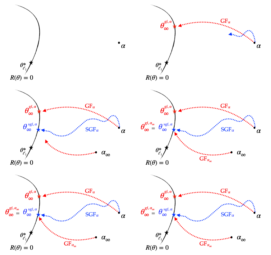
Figure 5: Illustration of the different implicit regularisations (part 1): SGD converges towards a solution which is the same as that of GD but which has been initialised with a strictly smaller scale, making it closer to the minimum \(\ell_1\)-norm solution.

Finally note that the magnitude of the effect of stochasticity on the implicit regularisation problem is linked with the convergence speed of the training loss through \(\int_0^\infty \mathcal{R}(\beta_s) \text{d}s\): the slower the training speed, the bigger this integral, and the closer the recovered solution is to the minimum \(\ell_1\)-norm interpolator.

Now what if, in addition to the inherent stochasticity, we inject deliberately some artificial noise to have “\(\int_0^\infty \mathcal{R}(\beta_s) \text{d}s = +\infty\)”? This would lead to “\(\alpha_\infty \to 0\)” and the retrieved interpolator should exactly be the minimum \(\ell_1\) norm interpolator! To make this statement rigorous, more work is needed [19], but under a few more assumptions it can be shown that indeed, as could be expected, when label noise is added then the iterates concentrate around the minimum \(\ell_1\)-norm interpolator. Here is a sketch of what we proved for this system:

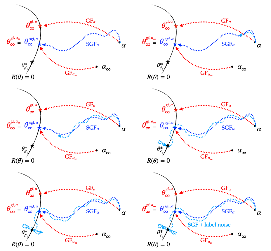
Figure 6: Illustration of the different implicit regularisations (part 2): if label noise is added, the iterates do not converge but concentrate around the minimum \(\ell_1\)-norm interpolator.

Beyond good and evil

Up until now, we have exhibited an algorithmic implicit bias which depends on the architecture and the algorithm. However keep in mind that this not a value-judgment of any kind! It is incorrect to think that a certain regularisation is “universally better” than another. It all depends on the setting and on the structure of the “true” distribution we want to learn. To make this clear, we provide an example which highlights this.

Assume we have a dataset \((x_i, y_i)_{i \leq n} \in \mathbb{R} \times \mathbb{R}\) where each sample is drawn from an unknown distribution \(\mathcal{D}\). Assume that \(\mathcal{D}\) is such that \(y = f^*(x)\) for some function \(f^* : \mathbb{R} \to \mathbb{R}\). In order to construct a prediction function from our samples, we consider performing linear regression using a feature map: \(f_\beta(x) = \langle \beta, \phi(x) \rangle\) where \(\phi(x) = (\frac{1}{k} \cos(2\pi k x), \frac{1}{k} \sin(2\pi k x))_{k \leq d/2} \in \mathbb{R}^d\). Assuming that \(d\) is larger than \(n\), there exists an infinity of interpolators \(\beta^*\) such that for all \(i \leqslant n\), \(f_{\beta^*}(x_i) = y_i\). Amongst all of these, lets have a look at the minimum \(\ell_1\)-norm and \(\ell_2\)-norm interpolators. As seen in the following two figures, depending on the distribution \(\mathcal{D}\) we consider, the generalisation performances of the min-\(\ell_1\) and min-\(\ell_2\) norms are very different.

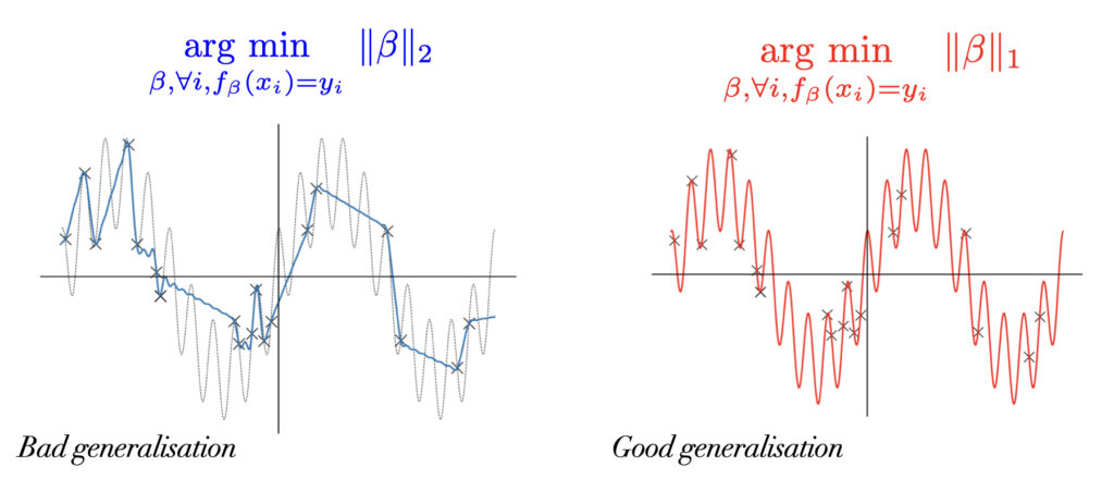
Figure 7: The minimum \(\ell_1\)-norm interpolator generalises much better than the minimum \(\ell_2\). \(f^*: \mathbb{R} \to \mathbb{R}\) is the sum of \(2\) sinusoids and is represented by the dotted black lines. Each black cross corresponds to a training sample \((x_i, y_i) \in \mathbb{R} \times \mathbb{R}\).

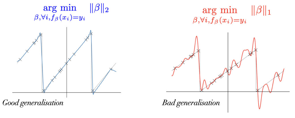
Figure 8: The minimum \(\ell_2\)-norm interpolator generalises much better than the minimum \(\ell_1\) norm. \(f^*: \mathbb{R} \to \mathbb{R}\) is the sum of an infinity of sinusoids and is represented by the dotted black lines. Each black cross corresponds to a training sample \((x_i, y_i) \in \mathbb{R} \times \mathbb{R}\).

Hence understanding the implicit bias of an algorithm on a given architecture is only a part of the big picture since it only brings out the structure of the recovered interpolators. The remaining part is to try and understand why these implicit regularisation are indeed “good” for our real world datasets. This is what is explored in the benign overfitting literature [26, 27].

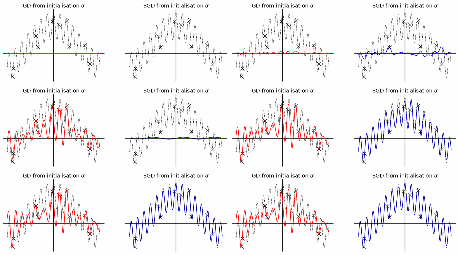
Before wrapping this blog-post up, let us provide one final toy example which highlights the advantage of SGD over GD when it comes to recovering a sparse solution. Assume we consider a similar feature map as before but now we use the diagonal parametrisation: \(f_\theta(x) = \langle u \odot v, \phi(x) \rangle\) where \(\phi(x) = (\cos(2\pi k x), \sin(2\pi k x))_{k \leq d/2} \in \mathbb{R}^d\). Instead of directly considering the minimum norm solutions, we perform GD and SGD (with a bit of label noise to boost the effect) with a same initialisation scale \(\alpha\). As you can observe the solution obtained by gradient descent is not sparse enough to perfectly recover the true \(f^*\), this is because \(\alpha\) is not small enough and therefore \(\phi_\alpha\) is not close enough to the \(\ell_1\) norm. However SGD performs much better and is able to recover pretty well the true distribution due to \(\phi_{\alpha_\infty} \sim \Vert \cdot \Vert_1\)!

Conclusion

In this blog post, we introduced the notion of algorithmic regularisation, a concept which is key in order to understand the current success of deep neural networks. We started with a simple linear parametrisation in order to clarify the notion before moving to a toy neural network which already conveys many of the characteristics of more sophisticated networks. For such a network, we saw that the initialisation scale and SGD’s noise play a fundamental role in the structure of the recovered estimator. In order to uncover the implicit regularisation problem, we heavily relied on mirror-like dynamics followed by the predictor flow \((\beta_t)_{t \geq 0}\). It is natural to want to try to use such convenient tools for more complicated architectures.
Unfortunately there exists some negative results showing that the re-parametrisation of a gradient flow cannot in general be written as a mirror flow [20, 21]. It would be interesting to find less restrictive frameworks than mirror structures which still enable a clean characterisation of algorithmic biases for more complex architectures. For example, there exists works such as [22, 23] which use very different tools but for which unnecessarily strong assumptions on the data are required. We can only imaging how much more challenging it will be to take the effect of noise into account, there is still a long but exciting journey ahead!

Aknowledgments. We would like to thank Nicolas Flammarion for guiding us on the project which is at the origin of this blog post, as well as Hadrien Hendrikx for proofreading it and making good clarifying suggestions.

References

[1] N.S. Keskar, D. Mudigere, J. Nocedal, M. Smelyanskiy and P.T.P. Tang. On large-batch training for deep learning: Generalization gap and sharp minima. In International Conference on Learning Representations (ICLR), 2017.
[2] Y. Cooper. The loss landscape of overparameterized neural networks. Technical Report, arXiv:1804.10200, 2018.
[3] Chiyuan Zhang, Samy Bengio, Moritz Hardt, Benjamin Recht, and Oriol Vinyals. Understanding deep learning requires rethinking generalization. In International Conference on Learning Representations, 2017.
[4] D. Soudry, E. Hoffer, M. S. Nacson, S. Gunasekar, and N. Srebro. The implicit bias of gradient descent on separable data. The Journal of Machine Learning Research, 19(1):2822–2878, 2018.
[5] L. Chizat and F. Bach. Implicit bias of gradient descent for wide two-layer neural networks trained with the logistic loss. In Conference on Learning Theory, pages 1305–1338. 2020.
[6] Z. Ji and M. Telgarsky. Gradient descent aligns the layers of deep linear networks. In International Conference on Learning Representations, 2019.
[7] F. Bach. Learning Theory from first principles. Draft Book, 2022.
[8] B. Lemaire, An asymptotical variational principle associated with the steepest descent method for a convex function, Journal of Convex Analysis, Vol.3, n°1, 1996,63-70.
[9] T. Vaskevicius, V. Kanade, and P. Rebeschini. Implicit regularization for optimal sparse recovery. Advances in Neural Information Processing Systems, 32, 2019.
[10] B. Woodworth, S. Gunasekar, J. D. Lee, E. Moroshko, P. Savarese, I. Golan, D. Soudry, and N. Srebro. Kernel and rich regimes in overparametrized models. In Conference on Learning Theory, pages 3635–3673. 2020.
[11] A. S. Nemirovski and D. B. Yudin, Problem Complexity and Method Efficiency in Optimization. New York: Wiley, 1983.
[12] A. Beck and M. Teboulle. Mirror descent and nonlinear projected subgradient methods for convex optimization. Operations Research Letters, 2003.
[13] F. Alvarez, J. Bolte, and O. Brahic. Hessian Riemannian gradient flows in convex programming. SIAM Journal on Control and Optimization, 43(2):477–501, 2004.
[14] S. Gunasekar, J. Lee, D. Soudry, and N. Srebro. Characterizing implicit bias in terms of optimization geometry. In Proceedings of the International Conference on Machine Learning, volume 80, pages 1832–1841, 2018.
[15] L. Chizat, E. Oyallon, and F. Bach. On lazy training in differentiable programming. In Advances in Neural Information Processing Systems, volume 32, 2019.
[16] S. Wojtowytsch. Stochastic gradient descent with noise of machine learning type. Part I: Discrete time analysis Technical Report, arXiv-2105.01650, 2021.
[17] S. Jastrzebski, Z. Kenton, D. Arpit, N. Ballas, A. Fischer, Y. Bengio, and A. Storkey. Three factors influencing minima in SGD. Technical report, arXiv:1711.04623, 2017.
[18] S. Pesme, L. Pillaud-Vivien, and N. Flammarion. Implicit bias of sgd for diagonal linear networks: a provable benefit of stochasticity. Advances in Neural Information Processing Systems, 34:29218–29230, 2021.
[19] L. Pillaud-Vivien, J. Reygner, and N. Flammarion. Label noise (stochastic) gradient descent implicitly solves the lasso for quadratic parametrisation. In Conference on Learning Theory, pages 2127–2159, 2022.
[20] S. Gunasekar, B. Woodworth, N. Srebro. Mirrorless mirror descent: A natural derivation of mirror descent. In International Conference on Artificial Intelligence and Statistics. 2021.
[21] Z. Li, T. Wang, J.D. Lee, S. Arora, Implicit Bias of Gradient Descent on Reparametrized Models: On Equivalence to Mirror Descent. Technical report, arXiv:2207.04036, 2022.
[22] S. Gunasekar, B. Woodworth, S. Bhojanapalli, B. Neyshabur, and N. Srebro. Implicit regularization in matrix factorization. In Advances in Neural Information Processing Systems, pages 6152–6160, 2017.
[23] E. Boursier, L. Pillaud-Vivien, N. Flammarion. Gradient flow dynamics of shallow ReLU networks for square loss and orthogonal inputs. Technical report, arXiv:2206.00939, 2022.
[24] J. Z. HaoChen, C. Wei, J. D. Lee, T. Ma. Shape Matters: Understanding the Implicit Bias of the Noise Covariance. In Conference on Learning Theory, 2021.
[25] D. Masters and C. Luschi. Revisiting small batch training for deep neural networks. arXiv-1804.07612, 2018.
[26] P. Bartlett, P. M. Long, G. Lugosi, A. Tsigler. Benign overfitting in linear regression. In Proceedings of the National Academy of Sciences, 2021.
[27] M. Belkin, A. Rakhlin, A. B. Tsybakov. Does data interpolation contradict statistical optimality? In Proceedings of the International Conference on Artificial Intelligence and Statistics, 2019.
Details on how to obtain the mirror flow from the gradient flow
Recall that the gradient flow on the diagonal linear network, from an initial point \((u_{t = 0}, v_{t=0}) = (u_0, v_0) \in \mathbb{R}^{2d}\) writes: $$ \dot u_t = \ – \frac{1}{n} [X^{\top} r_t] \odot v_t \quad \mathrm{and} \quad \dot v_t = \ – \frac{1}{n} [X^{\top} r_t] \odot u_t, $$ where \(r_t := X (u_t \odot v_t)\, – y = X \beta_t \, – y \in \mathbb{R}^n\) is the residual vector at time \(t\) and \(\beta_t = u_t \odot v_t\). To obtain the flow which is followed by the predictors, we simply differentiate \(\beta_t\) and get: $$ \dot{\beta}_t = \ – \frac{1}{n} [X^{\top} r_t] \odot (u_t^2 + v_t^2) $$ where the square must be understood element-wise. Here it may seem that we are stuck as \((u, v) \mapsto u \odot v\) is not bijective hence it could be impossible to write \(u_t^2 + v_t^2 \) as a function of \(\beta_t\). However due to the invariance \((\lambda \odot u) \odot (v / \lambda) = u \odot v\) for \(\lambda \in \mathbb{R}^d\) which appears in our network, we have that along the flow, \(u_t^2 – v_t^2\) is a conserved quantity (we can also simply differentiate the quantity and notice that the derivative is equal to \(0\) but it is more principled to see this as a conserved quantity due to the invariance in our architecture). This property is often called the “balancedness” property and holds for more complex architectures as soon as there exists a similar invariance. Recall that for simplicity we assumed that we initialise the weights as \(u_{t = 0} = \alpha \mathbf{1} \in \mathbb{R}^d\) and \(v_{t = 0} = \mathbf{0} \in \mathbb{R}^d\).
Back to our \((\beta_t)_t\) flow: equipped with this conserved quantity \(u_t^2 – v_t^2 = \alpha^2\) (where we abuse the notation \(\alpha := \alpha \mathbf{1}\)), we can now write \(u_t^2 + v_t^2 = \sqrt{4 \beta_t^2 + \alpha^4}\) and therefore $$ \dot{\beta}_t = \ – \frac{1}{n} [X^{\top} r_t] \odot \sqrt{4 \beta_t^2 + \alpha^4} = \ – \sqrt{4 \beta_t^2 + \alpha^4} \odot \nabla_\beta \mathcal{R}(\beta_t),$$ since \(\nabla_\beta \mathcal{R}(\beta) = \frac{1}{n} X^\top (X \beta – y) = \frac{1}{n} X^\top r(\beta)\). The sharpest eyes will notice that by letting \(\phi_\alpha : \mathbb{R}^d \to \mathbb{R}\) with $$\begin{aligned} \phi_\alpha(\beta) &= \frac{1}{4} \sum_{i=1}^d \Big ( 2 \beta_i \mathrm{arcsinh}( \frac{2 \beta_i}{\alpha^2} ) \ – \sqrt{4 \beta_i^2 + \alpha^4} + \alpha^2 \Big ) \\ \nabla_\beta \phi_\alpha(\beta) &= \frac{1}{2} \mathrm{arcsinh}(\frac{2 \beta}{\alpha^2}) \in \mathbb{R}^d \\ \nabla_\beta^2 \phi_\alpha(\beta) &= \mathrm{diag} \left[1 / \sqrt{4 \beta_i^2 + \alpha^4}\right]_{i = 1}^{d} \in \mathbb{R}^{d \times d}. \end{aligned}$$ Which means that we can write \(\dot{\beta}_t = \ – \nabla^2 \phi_\alpha(\beta_t)^{-1} \nabla_\beta \mathcal{R}(\beta_t)\) which can also be seen as
$$\frac{\mathrm{d}}{\mathrm{d} t} \nabla \phi_\alpha(\beta_t) = \ – \nabla_\beta \mathcal{R}(\beta_t) .$$ This is exactly the mirror flow equation with potential \(\phi_\alpha\).
Very interesting, as always, thanks a lot !
But a central assumption is the overparameterized regime: I’m not so sure this is really the regime of most DNNs? For instance, Bloom, one of the largest model, has 175B parameters, but it has been trained on “1.6TB of pre-processed text, converted into 350B unique tokens”. I’ve got the feeling that it’s not the only one, and that many DNNs in NLP are not far but stay below the interpolation threshold? Did I miss something or are there other common DNNs that clearly are overparameterized?
(I didn’t check for the mixture-of-experts-DNN, where the number of parameters scale quickly, but they’re a bit special as all parameters are not used at the same time…)
Thanks for your remark! Sure, we aren’t in 2016 (https://arxiv.org/abs/1611.03530) anymore… however, the story about understanding the implicit bias it also the story of trying to understand the dynamics and the structure of predictors retrieved. Even tough we are not in the interpolation regime for these tasks, maybe such studies can still provide us insights on the role of the architecture, the initialization, SGD’s noise etc.