The many faces of integration by parts – I : Abel transformation

Integration by parts is a highlight of any calculus class. It leads to multiple classical applications for integration of logarithms, exponentials, etc., and it is the source of an infinite number of exercises and applications to special functions. In this post, I will look at a classical discrete extension that is useful in machine learning and optimization, namely Abel transformation, with applications to convergence proofs for the (stochastic) subgradient method. Next month, extensions to higher dimensions will be considered, with applications to score functions [2, 3] and randomized smoothing [4, 5].

Abel transformation: from continuous to discrete

The most classical version of integration by parts goes as follows. Given two continuously differentiable functions from \(\mathbb{R}\) to \(\mathbb{R}\), we have: $$ \int_a^b \!\!\!\!f(x)g'(x) dx = \Big[ f(x) g(x) \Big]_a^b \!-\! \int_a^b\!\!\! \!f'(x) g(x) dx = f(b) g(b)\, – f(a)g(a)-\! \int_a^b\! \!\!\! f'(x) g(x) dx.$$ This is valid for less regular functions, but this is not the main concern here. The proof follows naturally from the derivative of a product, but there is a nice “proof without words” (see, e.g., [1, p. 42] or here).

There is a discrete analogue referred to as Abel transformation or summation by parts, where derivatives are replaced by increments: given two real-valued sequences \((a_n)_{n \geq 0}\) and \((b_n)_{n \geq 0}\) (the second sequence could also be taken vector-valued), we can expand $$ \sum_{k=1}^n a_k ( b_k\, – b_{k-1}) =\sum_{k=1}^n a_k b_k \ – \sum_{k=1}^n a_k b_{k-1} = \sum_{k=1}^n a_k b_k \ – \sum_{k=0}^{n-1} a_{k+1} b_{k},$$ using a simple index increment in the second sum. Rearranging terms, this leads to $$ \sum_{k=1}^n a_k ( b_k\, – b_{k-1}) = a_n b_n \ – a_0 b_0\ – \sum_{k=0}^{n-1} ( a_{k+1} – a_{k } ) b_k.$$ In other words, we can transfer the first-order difference from the sequence \((b_k)_{k \geq 0}\) to the sequence \((a_k)_{k \geq 0}\). A few remarks:

• Warning! It is very easy/common to make mistakes with indices and signs.
• I gave the direct proof but a proof through explicit integration by part is also possible, by introducing the piecewise-constant function \(f\) equal to \(a_k\) on \([k,k+1)\), and \(g\) continuous piecewise affine equal to \(b_{k} + (t-k) ( b_{k+1}-b_{k})\) for \(t \in [k,k+1]\), and integrating between \(0+\) and \(n+\).

There are classical applications for the convergence of series (see here), but in this post, I will show how it can lead to an elegant result for stochastic gradient descent for non-smooth functions and decaying step-sizes.

Decaying step-sizes in stochastic gradient descent

The Abel summation formula is quite useful when analyzing optimization algorithms, and we give a simple example below. We consider a sequence of random potentially non-smooth convex functions \((f_k)_{k \geq 0}\) which are independent and identically distributed functions from \(\mathbb{R}^d \) to \(\mathbb{R}\), with expectation \(F\). The goal is to find a minimizer \(x_\ast\) of \(F\) over a some convex bounded set \(\mathcal{C}\), only being given access to some stochastic gradients of \(f_k\) at well-chosen points. The most classical example is supervised machine learning, where \(f_k(\theta)\) is the loss of a random observation for the predictor parameterized by \(\theta\). The difficulty here is the potential non-smoothness of the function \(f_k\) (e.g., for the hinge loss and the support vector machine).

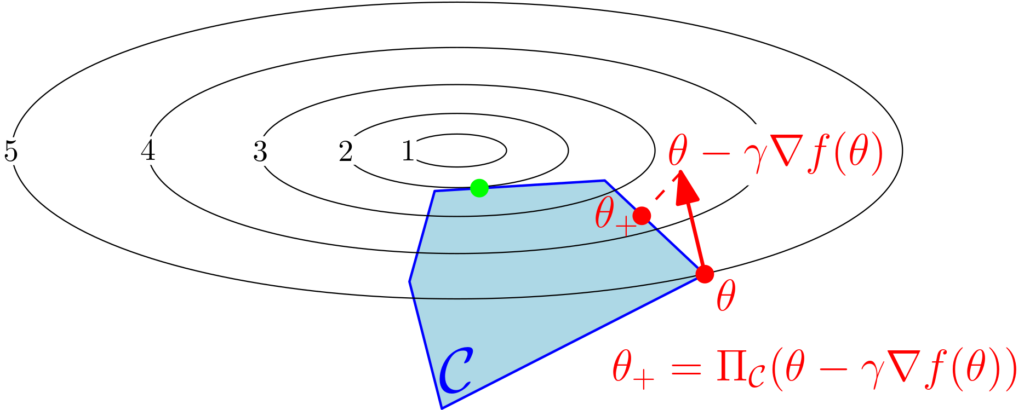
We consider the projected stochastic subgradient descent method. The deterministic version of this method dates back to Naum Shor [6] in 1962 (see nice history here). The method goes as follows: starting from some \(\theta_0 \in \mathbb{R}^d\), we perform the iteration $$ \theta_{k} = \Pi_{ \mathcal{C} } \big( \theta_{k-1} – \gamma_k \nabla f_k(\theta_{k-1}) \big),$$ where \(\Pi_{ \mathcal{C}}: \mathbb{R}^d \to \mathbb{R}^d\) is the orthogonal projection onto the set \(\mathcal{C}\), and \(\nabla f_k(\theta_{k-1})\) is any subgradient of \(f_k\) at \(\theta_{k-1}\).

We make the following standard assumptions: (a) the set \(\mathcal{C}\) is convex and compact with diameter \(\Delta\) (with respect to the \(\ell_2\)-norm), (b) the functions \(f_k\) are almost surely convex and \(B\)-Lipschitz-continuous (or equivalently with gradients bounded in \(\ell_2\)-norm by \(B\)). We denote by \(\theta_\ast\) a minimizer of \(f\) on \(\mathcal{C}\) (there can be multiple ones).

For non-smooth problems, choosing a constant step-size does not lead to an algorithm converging to a global minimizer: decaying step-sizes are then needed.

Convergence proof through Lyapunov functions

Since the functions \(f_k\) are non-smooth, we cannot use Taylor expansions, and we rely on a now classical proof technique dating back from the 1960’s (see, e.g., a paper by Boris Polyak [7] in Russian), that has led to several extensions in particular for online learning [8]. The proof relies on the concept of “Lyapunov functions“, often also referred to as “potential functions”. This is a non-negative function \(V(\theta_k)\) of the iterates \(\theta_k\), that is supposed to go down along iterations (at least in expectation). In optimization, standard Lyapunov functions are \(V(\theta) = F(\theta)\, – F(\theta_\ast)\) or \(V(\theta) = \| \theta \ – \theta_\ast\|_2^2\).

For the subgradient method, we will not be able to show that the Lyapunov function is decreasing, but this will lead through a manipulation which is standard in linear dynamical system analysis to a convergence proof for the averaged iterate: that is, if \(V(\theta_k) \leqslant V(\theta_{k-1})\ – W(\theta_{k-1}) + \varepsilon_k\), for a certain function \(W\) and extra positive terms \(\varepsilon_k\), then, using telescoping sums, $$ \frac{1}{n} \sum_{k=1}^n W(\theta_{k-1}) \leqslant \frac{1}{n} \big( V(\theta_0)\ – V(\theta_n) \big) + \frac{1}{n} \sum_{k=1}^n \varepsilon_k.$$ We can then either use Jensen’s inequality to get a bound on \(W \big( \frac{1}{n} \sum_{k=1}^n \theta_{k-1} \big)\), or directly get a bound on \(\min_{k \in \{1,\dots,n\}} W(\theta_{k-1})\). The first solution gives a performance guarantee for a well-defined iterate, while the second solution only shows that among the first \(n-1\) iterates, one of them has a performance guarantee; in the stochastic set-up where latex \(W\) is an expectation, it is not easily possible to know which one, so we will consider only averaging below.

Standard inequality. We have, by contractivity of orthogonal projections: $$ \|\theta_k \ – \theta_\ast\|_2^2 = \big\| \Pi_{ \mathcal{C} } \big( \theta_{k-1} – \gamma_k \nabla f_k(\theta_{k-1}) \big) – \Pi_{ \mathcal{C} } (\theta_\ast) \big\|_2^2 \leqslant \big\| \theta_{k-1} – \gamma_k \nabla f_k(\theta_{k-1}) -\ \theta_\ast \big\|_2^2.$$ We can then expand the squared Euclidean norm to get: $$ \|\theta_k – \theta_\ast\|_2^2 \leqslant \|\theta_{k-1} – \theta_\ast\|_2^2 \ – 2\gamma_k (\theta_{k-1} – \theta_\ast)^\top \nabla f_k (\theta_{k-1}) + \gamma_k^2 \| \nabla f_k(\theta_{k-1})\|_2^2.$$ The last term is upper-bounded by \(\gamma_k^2 B^2\) because of the regularity assumption on \(f_k\). For the middle term, we use the convexity of \(f_k\), that is, the function \(f_k\) is greater than its tangent at \(\theta_{k-1}\). See figure below.

We then obtain $$ f_k(\theta_\ast) \geqslant f_k(\theta_{k-1}) + \nabla f_k(\theta_{k-1})^\top ( \theta_{\ast} – \theta_{k-1}).$$

Putting everything together, this leads to $$ \|\theta_k \ – \theta_\ast\|_2^2 \leqslant \|\theta_{k-1}\ – \theta_\ast\|_2^2 \ – 2\gamma_k \big[ f_k(\theta_{k-1}) \ – f_k(\theta_\ast) \big] + \gamma_k^2 B^2.$$ At this point, except the last term, all terms are random. We can now take expectations, with a particular focus on the term \(\mathbb{E} \big[ f_k(\theta_{k-1}) \big]\), for which we can use the fact that the random function \(f_k\) is independent from the past, so that $$ \mathbb{E} \big[ f_k(\theta_{k-1}) \big] = \mathbb{E} \Big[ \mathbb{E} \big[ f_k(\theta_{k-1}) \big| f_{1},\dots,f_{k-1} \big] \Big] =\mathbb{E} \big[ F(\theta_{k-1}) \big] . $$ We thus get $$ \mathbb{E} \big[ \|\theta_k – \theta_\ast\|_2^2\big] \leqslant \mathbb{E} \big[ \|\theta_{k-1} – \theta_\ast\|_2^2\big] – 2\gamma_k \big( \mathbb{E} \big[ F(\theta_{k-1}) \big] – F(\theta_\ast) \big) + \gamma_k^2 B^2.$$ As above, we can now isolate the excess in function values as: $$ \mathbb{E} \big[ F(\theta_{k-1}) \big] – F(\theta_\ast) \leqslant \frac{1}{2 \gamma_k} \Big( \mathbb{E} \big[ \|\theta_{k-1} – \theta_\ast\|_2^2\big] – \mathbb{E} \big[ \|\theta_{k} – \theta_\ast\|_2^2\big] \Big) + \frac{\gamma_k}{2} B^2.$$ At this point, the “optimization part” of the proof is done. Only algebraic manipulations are needed to obtain a convergence rate. This is where Abel transformation will come in.

From fixed horizon to anytime algorithms

The lazy way. At this point, many authors (including me sometimes) will take a constant step-size \(\gamma_k = \gamma\) so as to obtain a telescopic sum, leading to $$ \frac{1}{n} \sum_{k=1}^n \mathbb{E} \big[ F(\theta_{k-1}) \big] – F(\theta_\ast) \leqslant \frac{1}{2n\gamma} \Big( \mathbb{E} \big[ \|\theta_{0} \ – \theta_\ast\|_2^2\big] – \mathbb{E} \big[ \|\theta_{n}\ – \theta_\ast\|_2^2\big] \Big) + \frac{\gamma}{2} B^2,$$ which is less than \(\displaystyle \frac{\Delta^2}{2n \gamma} + \frac{\gamma}{2} B^2\), and minimized for \(\displaystyle \gamma = \frac{ \Delta}{B \sqrt{n}}\), leading to a convergence rate less than \(\displaystyle \frac{ B \Delta}{\sqrt{n}}\). Using Jensen’s inequality, we then get for \(\bar{\theta}_n = \frac{1}{n} \sum_{k=1}^n \theta_{k-1}\): $$\mathbb{E} \big[ F(\bar{\theta}_{n}) \big] – F(\theta_\ast) \leqslant \frac{ B \Delta}{\sqrt{n}} .$$ This result leads to the desired rate but can be improved in at least one way: the step-size currently has to depend on the “horizon” \(n\) (which has to be known in advance), and the algorithm is not “anytime”, which is not desirable in practice (where one often launches an algorithm and stops it when it the performance gains have plateaued or when the user gets bored waiting).

Non-uniform averaging. Another way [9] is to consider the non-uniform average $$ \eta_{k} = \frac{\sum_{k=1}^n \gamma_{k} \theta_{k-1}}{\sum_{k=1}^n \gamma_{k}}, $$ for which telescoping sums apply as before, to get $$ \mathbb{E} \big[ F(\eta_k) \big] – F(\theta_\ast) \leqslant \frac{1}{2} \frac{\Delta^2 + B^2 \sum_{k=1}^n \gamma_k^2}{\sum_{k=1}^n \gamma_{k}}.$$ Then, by selecting a decaying step-size \(\displaystyle \gamma_k = \frac{ \Delta}{B \sqrt{k}}\), that depends on the iteration number, we get a rate proportional to \(\displaystyle \frac{ B \Delta}{\sqrt{n}} ( 1 + \log n)\). We now have an anytime algorithm, but we have lost a logarithmic term, which is not the end of the world, but still disappointing. In [9], “tail-averaging” (only averaging iterates between a constant times \(n\) and \(n\)) is proposed, that removes the logarithmic term but requires to store iterates (moreover, the non-uniform averaging puts too much weight on the first iterates, slowing down convergence).

Using Abel transformation. If we start to sum inequalities from \(k=1\) to \(k=n\), we get, with \(\delta_k = \mathbb{E} \big[ \|\theta_{k} – \theta_\ast\|_2^2\big]\) (which is always between \(0\) and \(\Delta^2\)): $$ \frac{1}{n} \sum_{k=1}^n \mathbb{E} \big[ F(\theta_{k-1}) \big] – F(\theta_\ast) \leqslant \frac{1}{n} \sum_{k=1}^n \bigg( \frac{1}{2 \gamma_k} \Big( \delta_{k-1} – \delta_k \Big)\bigg) + \frac{1}{n} \sum_{k=1}^n \frac{\gamma_k}{2} B^2,$$ which can be transformed through Abel transformation into $$ \frac{1}{n} \sum_{k=1}^n \mathbb{E} \big[ F(\theta_{k-1}) \big] – F(\theta_\ast) \leqslant \frac{1}{n} \sum_{k=1}^{n-1} {\delta_k} \bigg(\frac{1}{ 2 \gamma_{k+1}}- \frac{1}{ 2 \gamma_{k}} \bigg) + \frac{\delta_0}{2 n \gamma_1}- \frac{\delta_t}{2 n \gamma_t}+ \frac{1}{n} \sum_{k=1}^n \frac{\gamma_k}{2} B^2.$$ For decreasing step-size sequences, this leads to $$ \frac{1}{n} \sum_{k=1}^n \mathbb{E} \big[ F(\theta_{k-1}) \big] – F(\theta_\ast) \leqslant \frac{1}{n} \sum_{k=1}^{n-1} {\Delta^2} \bigg(\frac{1}{ 2\gamma_{k+1}}- \frac{1}{ 2\gamma_{k}} \bigg) + \frac{\Delta^2}{2n \gamma_1}+ \frac{1}{n} \sum_{k=1}^n \frac{\gamma_k}{2} B^2,$$ and thus $$ \frac{1}{n} \sum_{k=1}^n \mathbb{E} \big[ F(\theta_{k-1}) \big] – F(\theta_\ast) \leqslant \frac{\Delta^2 }{2 n \gamma_n} + \frac{1}{n} \sum_{k=1}^n \frac{\gamma_k}{2} B^2.$$ For \(\gamma_k = \frac{ \Delta}{B \sqrt{k}}\), this leads to an upper bound $$\frac{\Delta B }{2 \sqrt{n}} \big( 1+ \frac{1}{\sqrt{n}} \sum_{k=1}^n \frac{1}{\sqrt{k}}\big) \leqslant \frac{3 \Delta B }{2 \sqrt{n}},$$ which is up to a factor \(\frac{3}{2}\) exactly the same bound as with a constant step-size, but now with an anytime algorithm.

Experiments

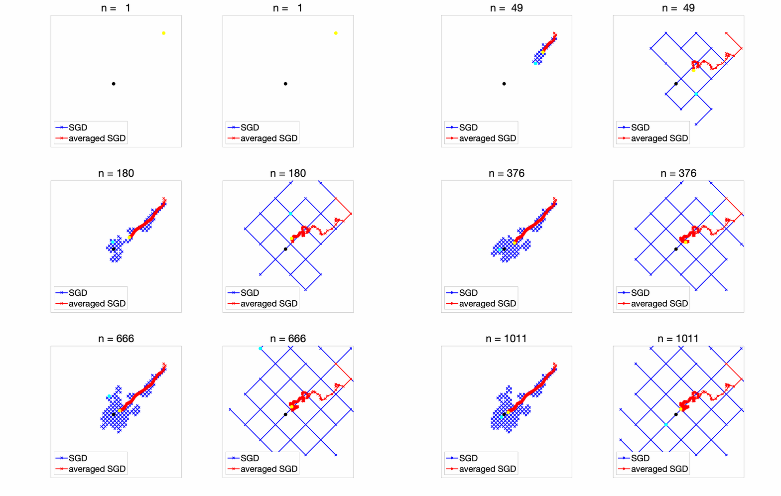
To illustrate the behaviors above, let’s consider minimizing \(\mathbb{E}_x \| x – \theta \|_1\), with respect to \(\theta\), with \(f_k(\theta) = \| x_k- \theta\|_1\), where \(x_k\) is sampled independently from a given distribution (here independent log-normal distributions for each coordinate). The global optimum \(\theta_\ast\) is the per-coordinate median of the distribution of \(x\)’s.

When applying SGD, the chosen subgradient of \(f_k\) has components in \(\{-1,1\}\). Hence in the plots below in two dimensions, the iterates are always on a grid. With a constant step-size: if the \(\gamma\) is too large (right), there are large oscillations, while if \(\gamma\) is too small (left), optimization is too slow. Note that while the SGD iterate with a constant step-size is always oscillating, the averaged iterate converges to some point (which is not the global optimum, and is typically at distance \(O(\gamma)\) away from it [11]).

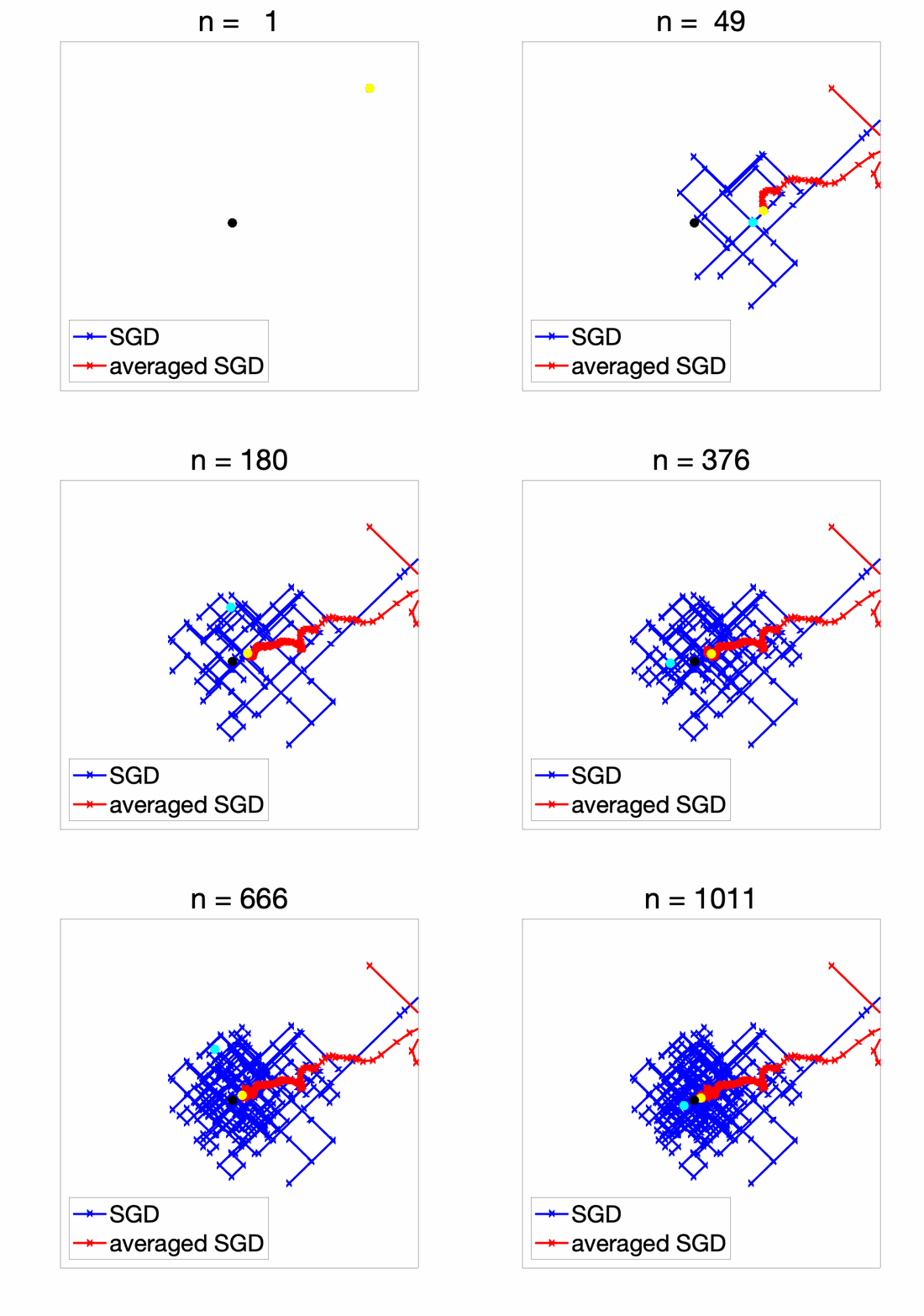
With a decaying step-size (figure below), the initial conditions are forgotten reasonably fast and the iterates converge to the global optimum (and of course, we get an anytime algorithm!).

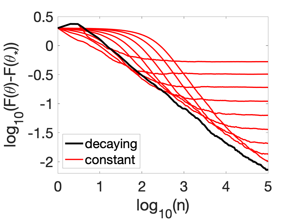
We can now compare in terms of function values, showing that a constant step-size only works well for a specific range of iteration numbers.

Conclusion

Being able to deal with decaying step-sizes and anytime algorithms is arguably not a major improvement, but quite a satisfactory one, at least to me! Discrete integration by parts is the key enabler here.

There is another rewarding aspect which is totally unrelated to integration by parts: when applied to supervised machine learning, we just obtained from elementary principles (convexity) and few calculations a generalization bound on unseen data, which is as good as regular bounds from statistics [10] that use much more complex tools such as Rademacher complexities (but typically no convexity assumptions): here, statistics considered independently from optimization is not only slower (considering the empirical risk and minimizing it using the plain non-stochastic subgradient method would lead to an \(n\) times slower algorithm) but also more difficult to analyze!

References

[1] Roger B. Nelsen, Proofs without Words: Exercises in Visual Thinking, Mathematical Association of America, 1997.
[2] Aapo Hyvärinen, Estimation of non-normalized statistical models by score matching. Journal of Machine Learning Research, 6(Apr), 695-709, 2005.
[3] Thomas M. Stoker, Consistent estimation of scaled coefficients.  Econometrica: Journal of the Econometric Society, 54(6):1461-1481, 1986.
[4] Tamir Hazan, George Papandreou, and Daniel Tarlow. Perturbation, Optimization, and Statistics. MIT Press, 2016.
[5] Quentin Berthet, Matthieu Blondel, Olivier Teboul, Marco Cuturi, Jean-Philippe Vert, Francis Bach, Learning with differentiable perturbed optimizers. Technical report arXiv 2002.08676, 2020.
[6] Naum Z. Shor. An application of the method of gradient descent to the solution of the network transportation problem. Notes of Scientific Seminar on Theory and Applications of Cybernetics and Operations Research, Ukrainian Academy of Sciences, Kiev, 9–17, 1962.
[7] Boris T. Polyak, A general method for solving extremal problems. Doklady Akademii Nauk SSSR, 174(1):33–36, 1967.
[8] Martin Zinkevich. Online convex programming and generalized infinitesimal gradient ascent. Proceedings of the international conference on machine learning )(ICML), 2003.
[9] Arkadi Nemirovski, Anatoli Juditsky, Guanghui Lan, Alexander Shapiro. Robust stochastic approximation approach to stochastic programming. SIAM Journal on optimization, 19(4):1574-1609, 2009.
[10] Stéphane Boucheron, Olivier Bousquet, Gabor Lugosi. Theory of classification: A survey of some recent advances. ESAIM: probability and statistics, 9, 323-375, 2005.
[11] Aymeric Dieuleveut, Alain Durmus, and Francis Bach. Bridging the gap between constant step size stochastic gradient descent and Markov chains. Annals of Statistics, 48(3):1348-1382, 2020.