The many faces of integration by parts – II : Randomized smoothing and score functions

This month I will follow-up on last month blog post and look at another application of integration by parts, which is central to many interesting algorithms in machine learning, optimization and statistics. In this post, I will consider extensions in higher dimensions, where we take integrals on a subset of \(\mathbb{R}^d\), and focus primarily on property of the so-called “score function” of a density \(p: \mathbb{R}^d \to \mathbb{R}\), namely the gradient of its logarithm: $$\nabla \log p(z) = \frac{1}{p(z)} \nabla p(z) \in \mathbb{R}^d,$$ or, done coordinate by coordinate, $$ \big(\nabla \log p(z)\big)_i = \frac{\partial [ \log p]}{\partial z_i}(z) = \frac{1}{p(z)} \frac{\partial p }{\partial z_i}(z) .$$ Note here that we take derivatives with respect to \(z\) and not with respect to some hypothetical external parameter, which is often the case in statistics (see here).

As I will show below, this quantity comes up in many different areas, most often used with integration by parts. After a short review on integration by parts and its applications to score functions, I will present four quite diverse applications, to (1) optimization and randomized smoothing, (2) differentiable perturbed optimizers, (3) learning single-index models in statistics, and (4) score matching for density estimation.

Integration by parts in multiple dimensions

I will focus only on situations where we have some random variable \(Z\) defined on \(\mathbb{R}^d\), with differentiable strictly positive density \(p(\cdot)\) with respect to the Lebesgue measure (I could also consider bounded supports, but then I would need to use the divergence theorem). I will consider a function \(f: \mathbb{R}^d \to \mathbb{R}\), and my goal is to provide an expression of \(\mathbb{E} \big[ f(Z) \nabla \log p(Z) \big] \in \mathbb{R}^d\) using the gradient of \(f\).

Assuming that \(f(z) p(z)\) goes to zero when \(\| z\| \to +\infty\), we have: $$\mathbb{E} \big[ f(Z) \nabla \log p(Z) \big] = \int_{\mathbb{R}^d} f(z)\Big( \frac{1}{p(z)} \nabla p (z) \Big) p(z) dz = \int_{\mathbb{R}^d} f (z) \nabla p(z) dz .$$ We can then use integration by parts (together with the zero limit at infinity), to get $$\int_{\mathbb{R}^d} f (z) \nabla p(z) dz = \ – \int_{\mathbb{R}^d} p (z) \nabla f(z) dz.$$ This leads to $$\mathbb{E} \big[ f(Z) \nabla \log p(Z) \big] =\ – \mathbb{E} \big[ \nabla f(Z) \big]. \tag{1}$$ In other words, expectations of the gradient of \(f\) can be obtained through expectations of \(f\) times the negative of the score function.

Note that Eq. (1) can be used in the two possible directions: to estimate the right hand side (expectation of gradients) when the score function is known, and vice-versa to estimate expectations (as a simple example, when \(f\) is constant equal to one, we get the traditional identity \(\mathbb{E} \big[ \nabla \log p(Z) \big] = 0\)).

Gaussian distribution. Assuming that \(p(z) = \frac{1}{(2\pi \sigma^2)^{d/2}} \exp\big( – \frac{1}{2 \sigma^2}\| z – \mu\|_2^2 \big)\), that is, \(Z\) is normally distributed with mean vector \(\mu \in \mathbb{R}^d\) and covariance matrix \(\sigma^2 I\), we get a particularly simple expression $$\frac{1}{\sigma^2} \mathbb{E} \big[ f(Z) (Z-\mu) \big] = \mathbb{E} \big[ \nabla f(Z) \big],$$ which is often referred to as Stein’s lemma (see for example an application to Stein’s unbiased risk estimation).

Vector extension. If now \(f\) has values in \(\mathbb{R}^d\), still with the product \(f(z) p(z)\) going to zero when \(\| z\| \to +\infty\), we get $$\mathbb{E} \big[ f(Z)^\top \nabla \log p(Z) \big] =\ – \mathbb{E} \big[ \nabla \!\cdot \! f(Z) \big], \tag{2}$$ where \(\nabla\! \cdot \! f\) is the divergence of \(f\) defined as \(\displaystyle \nabla\! \cdot\! f(z) = \sum_{i=1}^d \frac{\partial f}{\partial z_i}(z)\).

Optimization and randomized smoothing

We consider a function \(f: \mathbb{R}^d \to \mathbb{R}\), which is non-differentiable everywhere. There are several ways of smoothing it. A very traditional way is to convolve it with a smooth function. In our context, this corresponds to considering $$f_\varepsilon(x) = \mathbb{E} f(x+ \varepsilon Z) = \int_{\mathbb{R}^d} f(x+\varepsilon z) p(z) dz,$$ where \(z\) is a random variable with strictly positive sufficiently differentiable density, and \(\varepsilon \) is a positive parameter. Typically, if \(f\) is Lipschitz-continuous, \(| f – f_\varepsilon|\) is uniformly bounded by a constant times \(\varepsilon\).

Let us now assume that we can take gradients within the integral, leading to: $$\nabla f_\varepsilon(x) = \int_{\mathbb{R}^d} \nabla f(x+\varepsilon z) p(z) dz = \mathbb{E} \big[ \nabla f(x+\varepsilon z) \big].$$ This derivation is problematic as the whole goal is to apply this to functions \(f\) which are not everywhere differentiable, so the gradient \(\nabla f\) is not always defined. It turns out that when \(p\) is sufficiently differentiable, integration by parts exactly provides an expression which does not imply the gradient of \(f\).

Indeed, still imagining that \(f\) is differentiable, we can apply Eq. (1) to the function \(z \mapsto \frac{1}{\varepsilon} f(x+\varepsilon z)\), whose gradient is the function \(z \mapsto \nabla f(x+\varepsilon z)\), and get $$\nabla f_\varepsilon(x) = \ – \frac{1}{\varepsilon} \int_{\mathbb{R}^d} f(x+\varepsilon z) \nabla p(z) dz = \frac{1}{\varepsilon} \mathbb{E} \big[ – f(x+\varepsilon Z) \nabla \log p(Z)\big].$$ These computations can easily be made rigorous and we obtain an expression of the gradient of \(f_\varepsilon\) without invoking the gradient of \(f\) (see [23, 14] for details).

Moreover, if \(p\) is a differentiable function, we can expect the expectation in the right hand side of the equation above to be bounded, and therefore the function \(f_\varepsilon\) has gradients bounded by \(\frac{1}{\varepsilon}\).

This can be used within (typically convex) optimization in two ways:

• Zero-th order optimization: if our goal is to minimize the function \(f\), which is non-smooth, and for which we only have access to function values (so-called “zero-th order oracle), then we can obtain an unbiased stochastic gradient of the smoothed version \(f_\varepsilon\) as \(– f(x+\varepsilon z) \nabla \log p(z)\) where \(z\) is sampled from \(p\). The variance of the stochastic gradient grows with \(1/\varepsilon\) and the bias due to the use of \(f_\varepsilon\) instead of \(f\) is proportional to \(\varepsilon\). There is thus a sweet spot for the choice of \(\varepsilon\), with many variations; see, e.g., [5, 6, 7].
• Randomized smoothing with acceleration [8, 9]: Here the goal is to follow the “Nesterov smoothing” idea [10] and minimize a non-smooth function \(f\) using accelerated gradient descent on the smoothed version \(f_\varepsilon\), but this time with a stochastic gradient. Stochastic versions of Nesterov accelerations are then needed; this is useful when a full deterministic smoothing of \(f\) is too costly, see [11, 12] for details.

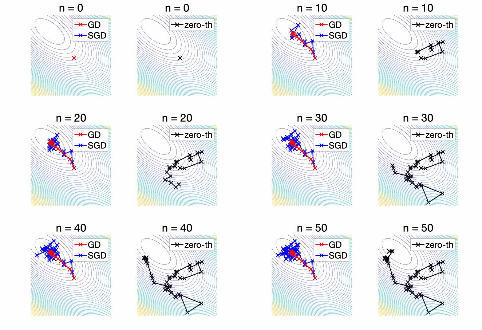
Example. We consider minimizing a quadratic function in two dimensions, and we compare below plain gradient descent, stochastic gradient descent (left) and zero-th order optimization where we take a step towards the direction \(– f(x+\varepsilon Z) \nabla \log p(Z)\) for a standard normal \(Z\). We compare stochastic zero-th order optimization to plain stochastic gradient descent (SGD) below: SGD is a first-order method requiring access to stochastic gradients with a variance that is bounded, while zero-th order optimization only requires function values, but with significantly higher variance and thus requiring more iterations to converge.

Differentiable perturbed optimizers

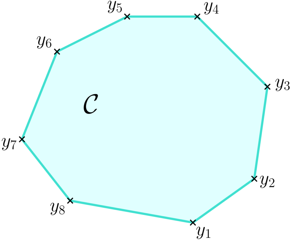
The randomized smoothing technique can be used in a different context with applications to differentiable programming. We now assume that the function \(f\) can be written as the support function of a polytope \(\mathcal{C}\), that is, for all \(u \in \mathbb{R}^d\), $$f(u) = \max_{y \in \mathcal{C}} u^\top y,$$ where \(\mathcal{C}\) is the convex hull of a finite family \((y_i)_{i \in I}\).

Typically, the family is very large (e.g., \(|I|\) is exponential in \(d\)), but a polynomial-time algorithm exists for computing an arg-max \(y^\ast(u)\) above. Classical examples, from simpler to more interesting, are:

• Simplex: \(\mathcal{C}\) is the set of vectors with non-negative components that sum to one, and is the convex hull of canonical basis vectors. Then \(f\) is the maximum function, and there are many classical ways of smoothing it (see link with the Gumbel trick below).
• Hypercube: \(\mathcal{C} = [0,1]^n\), which is the convex hull of all vectors in \(\{0,1\}^n\). The maximization of linear functions can then be done independently for each bit.
• Permutation matrices: \(\mathcal{C}\) is then the Birkhoff polytope, the convex hull of all permutation matrices (square matrices with elements in \(\{0,1\}\), and with exactly a single \(1\) in each row and column). Maximizing linear functions is the classical linear assignment problem.
• Shortest paths: given a graph, a path is a sequence of vertices which are connected to each other in the graph. They can classically be represented as a vector of of 0’s and 1’s indicating the edges which are followed by the paths. Minimizing linear functions is then equivalent to shortest path problems.

In many supervised applications, the vector \(u\) is as a function of some input \(x\) and some parameter vector \(\theta\). In order to learn the pararameter \(\theta\) from data, one needs to be able to differentiate with respect to \(\theta\), and this is typically done through the chain rule by differentiating \(y^\ast(u)\) with respect to \(u\). There come two immediate obstacles: (1) the element \(y^\ast(u)\) is not even well-defined when the arg-max is not unique, which is not a real problem because this can only be the case for a set of \(u\)’s with zero Lebesgue measure; and (2) the function \(y^\ast(u)\) is locally constant for most \(u\)’s, that is, the gradient is equal to zero almost everywhere. Thus, in the context of differentiable programming, this is non informative and essentially useless.

Randomized smoothing provides a simple and generic way to define an approximation which is differentiable and with informative gradient everywhere (there are others, such as adding a strongly convex regularizer \(\psi(y)\), and maximizing \(u^\top y\ – \psi(y)\) instead, see [20] for details. See also [24]).

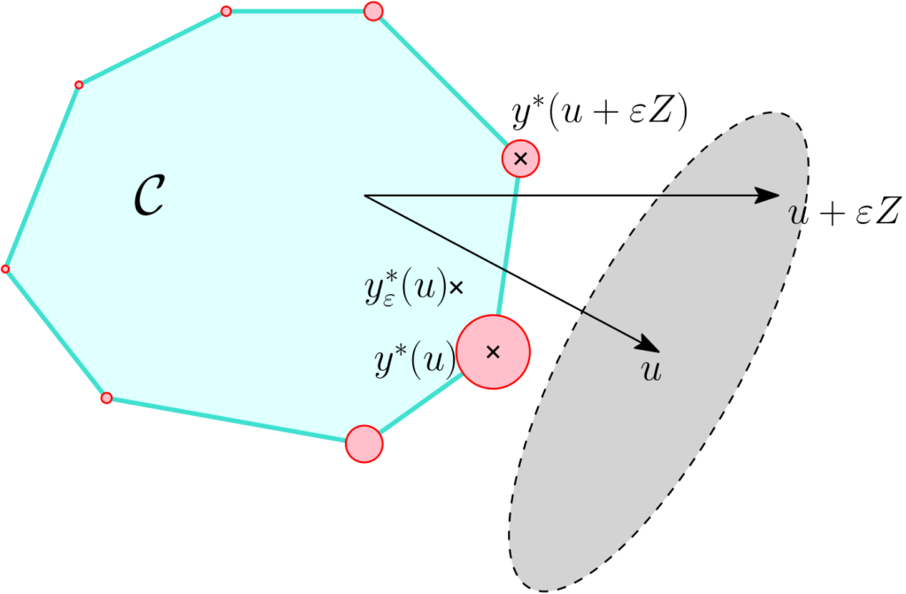
In order to obtain a differentiable function through randomized smoothing, we can consider \(y^\ast(u + \varepsilon z)\), for a random \(z\), which is an instance of the more general “perturb-and-MAP” paradigm [21, 22].

Since \(y^\ast(u)\) is a subgradient of \(f\) at \(u\) and \(f_\varepsilon(u) = \int_{\mathbb{R}^d} f(u+\varepsilon z) p(z) dz\), by swapping integration (with respect to \(z\)) and differentiation (with respect to \(u\)), we have the following identities: $$ \mathbb{E} \big[ y^\ast(u + \varepsilon Z) \big] = \nabla f_\varepsilon(u),$$ that is, the expectation of the perturbed arg-max is the gradient of the smoothed function \(f_\varepsilon\). I will use the notation \(y^\ast_\varepsilon(u) =\mathbb{E} \big[ y^\ast(u + \varepsilon Z) \big]\) to denote this gradient; see an illustration below.

In a joint work with Quentin Berthet, Mathieu Blondel, Oliver Teboul, Marco Cuturi, and Jean-Philippe Vert [14], we detail theoretical and practical properties of \(y^\ast_\varepsilon(u)\), in particular:

• Estimation: \(y^\ast_\varepsilon(u)\) can be estimated by replacing the expectation by empirical averages.
• Differentiability: if \(Z\) has a strictly positive density over \(\mathbb{R}^d\), then the function \(y^\ast_\varepsilon\) is infinitely differentiable, with simple expression of the Jacobian, obtained by integration by parts (see [23] for details).
• The Gumbel trick is the simplest instance of such a smoothing technique, with \(\mathcal{C}\) being the simplex, and \(Z\) having independent Gumbel distributions. The function \(f_\varepsilon\) is then a “log-sum-exp” function.

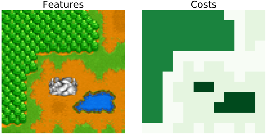
Illustration. Following [24], this can be applied to learn the travel costs in graphs based on features. The vectors \(y_i\) represent shortest path between the top-left and bottom-right corners, with costs corresponding to the terrain type. See [14] for details on the learning procedure. Here I just want to highlight the effect of varying the amount of smoothing characterized by \(\varepsilon\).

Learning single-index models

Given a random vector \((X,Y) \in \mathbb{R}^d \times \mathbb{R}\), we assume that \(Y = f(X) + \varepsilon\), where \(f(x) = \sigma(w^\top x)\) for some unknown function \(\sigma: \mathbb{R} \to \mathbb{R}\) and \(w \in \mathbb{R}^d\), with \(\varepsilon\) a zero-mean noise independent from \(X\). Given some observations \((x_1,y_1), \dots, (x_n,y_n)\) in \(\mathbb{R}^d \times \mathbb{R}\), the goal is to estimate the direction \(w \in \mathbb{R}^d\). This model is referred to as single-index regression models in the statistics literature [1, 2]

One possibility if \(\sigma\) was known would be to perform least-squares estimation and minimize with respect to \(w\) $$ \frac{1}{2n} \sum_{i=1}^n \big( y_i\ – \sigma(w^\top x_i) \big)^2, $$ which is a non-convex optimization problem in general. When \(\sigma\) is unknown, one could imagine adding the estimation of \(\sigma\) into the optimization, making it even more complicated.

Score functions provide an elegant solution that leads to the “average derivative method” (ADE) [3], which I will now describe. We consider \(p\) the density of \(X\). We then have, using Eq. (1): $$ \mathbb{E} \big[ Y \nabla \log p(X) \big] =\mathbb{E} \big[ f(X) \nabla \log p(X) \big] = \ – \mathbb{E} \big[ \nabla f(X) \big] =\ – \Big( \mathbb{E} \big[ \sigma'(w^\top X) \big] \Big) w, $$ which is proportional to \(w\). When replacing the expectation by an empirical mean, this provides a way to estimate \(w\) (up to a constant factor) without even knowing the function \(\sigma\), but assuming the density of \(X\) is known so that the score function is available.

Extensions. The ADE method can be extended in a number of ways to deal with more complex situations. Here are some examples below:

• Multiple index models: if the response/output \(Y\) is instead assumed of the form $$ Y = f(X) + \varepsilon = \sigma(W^\top x) + \varepsilon, $$ where \(W \in \mathbb{R}^{d \times k}\) is a matrix with \(k\) columns, we obtained a “multiple index model”, for which a similar technique seems to apply since now \(\nabla f(x) = W \nabla \sigma(W^\top x) \in \mathbb{R}^d\), and thus, for the assumed model \(\mathbb{E} \big[ Y \nabla \log p(X) \big]\) is in the linear span of the columns of \(W\); this is not enough for recovering the entire subspace if \(k>1\) because we have only a single element of the span. There are two solutions for this. The first one is is to condition on some values of \(Y\) being in some set \(\mathcal{Y}\), where one can show that \(\mathbb{E} \big[ Y \nabla \log p(X) | Y \in \mathcal{Y} \big]\) is also in the desired subspace; thus, with several sets \(\mathcal{Y}\), one can generate several elements, and after \(k\) of these, one can expect to estimate the full \(k\)-dimensional subspace. The idea of conditioning on \(Y\) is called sliced inverse regression [15], and the application to score function can be found in [16]. The second one is to consider higher-order moments and derivatives of the score functions, that is, using integration by parts twice! (see [17, 18, 16] for details).
• Neural networks: when the function \(\sigma\) is the sum of functions that depends on single variables, multiple-index models are exactly one-hidden-layer neural networks. Similar techniques can be used for deep networks with more than a single hidden layer (see [19]).

Moment matching vs. empirical risk minimization. In all cases mentioned above, the use of score functions can be seen as an instance of the method of moments: we assume a specific model for the data, derive identities satisfied by expectations of some functions under the model, and use these identities to identify a parameter vector. In the situations above, direct empirical risk minimization would lead to a potentially hard optimization problem. However, moment matching techniques rely heavily on the model being well-specified, which is often not the case in practice, while empirical risk minimization techniques try to fit the data as much as the model allows, and is thus typically more robust to model misspecification.

Score matching for density estimation

We consider the problem of density estimation. That is, given some observations \(x_1,\dots,x_n \in \mathbb{R}^d\) sampled independently and identically distributed from some distribution with density \(p\), we want to estimate \(p\) from the data. Given a model \(q_\theta \) with some parameters \(\theta\), the most standard method is maximum likelihood estimation, which corresponds to the following optimization problem: $$\max_{\theta \in \Theta} \frac{1}{n} \sum_{i=1}^n \log q_\theta(x_i).$$ It requires normalized densities that is, \(\int_{\mathbb{R}^d} q_\theta(x) dx = 1\), and dealing with normalized densities often requires to explicitly normalize them and thus to compute integrals, which is difficult when the underlying dimension \(d\) gets large.

Score matching is a recent method proposed by Aapo Hyvärinen [4] based on score functions. The simple (yet powerful) idea is to perform least-squares estimation on the score functions. That is, in the population case, the goal is to minimize $$\mathbb{E} \big\| \nabla \log p(X) \ – \nabla \log q_\theta(X) \big\|_2^2 = \int_{\mathbb{R}^d} \big\| \nabla \log p(x)\ – \nabla \log q_\theta(x) \big\|_2^2 p(x) dx.$$ Apparently, this expectation does not lead to an estimation procedure where \(p(x)\) is replaced by the empirical distribution of the data because of the presence of \(\nabla \log p(x)\). Integration by parts will solve this.

We can expand \(\mathbb{E} \big\| \nabla \log p(X) \ – \nabla \log q_\theta(X) \big\|_2^2\) as $$ \mathbb{E} \big\| \nabla \log p(X) \|_2^2 + \mathbb{E} \big\|\nabla \log q_\theta(X) \big\|_2^2 – 2 \mathbb{E} \big[ \nabla \log p(X)^\top \nabla \log q_\theta(X) \big]. $$ The first term is independent of \(q_\theta\) so it does not count when minimizing. The second term is an expectation with respect to \(p(\cdot)\) so it can be replaced by the empirical mean. The third term can be dealt with with integration by parts, that is Eq. (2), leading to: $$ – 2 \mathbb{E} \big[ \nabla \log p(X)^\top \nabla \log q_\theta(X) \big] = 2 \mathbb{E} \big[ \nabla \cdot \nabla \log q_\theta(X) \big] = 2 \mathbb{E} \big[ \Delta \log q_\theta(X) \big],$$ where \(\Delta\) is the Laplacian.

We now have an expectation with respect to the data distribution \(p\), and we can replace the expectation with an empirical average to estimate the parameter \(\theta\) from data \(x_1,\dots,x_n\). We then use the cost function $$\frac{1}{n} \sum_{i=1}^n \big\|\nabla \log q_\theta(x_i) \big\|_2^2 + \frac{2}{n} \sum_{i=1}^n \Delta \log q_\theta(x_i), $$ which is linear in \(\log q_\theta\). Hence, when the unnormalized log-density is linearly parameterized, which is common, we obtain a quadratic problem. This procedure has a number of attractive properties, in particular consistency [4], but the key benefit is to allow estimation without requiring normalizing constants.

Conclusion

Overall, the simple identity from Eq. (1), that is, \(\mathbb{E} \big[ f(Z) \nabla \log p(Z) \big] =\ – \mathbb{E} \big[ \nabla f(Z) \big]\), has many applications in diverse somewhat unrelated areas of machine learning, optimization and statistics. There are of course many other uses of integration by parts within this field. Feel free to add your preferred one as comment.

It has been a while since the last post on polynomial magic. I will revive the thread next month. I let you guess which polynomials will be the stars of my next blog post.

Acknowledgements. I would like to thank Quentin Berthet for producing the video of shortest paths, proofreading this blog post, and making good clarifying suggestions.

References

[1] James L. Powell, James H. Stock, Thomas M. Stoker. Semiparametric estimation of index coefficients. Econometrica: Journal of the Econometric Society. 57(6):1403-1430, 1989.
[2] Wolfgang Hardle, Peter Hall, Hidehiko Ichimura. Optimal smoothing in single-index models. Annals of Statistics. 21(1): 157-178(1993): 157-178.
[3] Thomas M. Stoker. Consistent Estimation of Scaled Coefficients. Econometrica, 54(6):1461-1481, 1986.
[4] Aapo Hyvärinen. Estimation of non-normalized statistical models by score matching. Journal of Machine Learning Research, 6(Apr), 695-709, 2005.
[5] Yurii Nesterov. Random gradient-free minimization of convex functions. Technical report, Université Catholique de Louvain (CORE), 2011.
[6] Boris T. Polyak and Alexander B. Tsybakov. Optimal order of accuracy of search algorithms in stochastic optimization. Problemy Peredachi Informatsii, 26(2):45–53, 1990.
[7] Abraham D. Flaxman, Adam Tauman Kalai, H. Brendan McMahan. Online convex optimization in the bandit setting: gradient descent without a gradient. In Proc. Symposium on Discrete algorithms (SODA), 2005.
[8] John C. Duchi, Peter L. Bartlett, and Martin J. Wainwright. Randomized Smoothing for Stochastic Optimization. SIAM Journal on Optimization, 22(2), 674–701, 2012.
[9] Alexandre d’Aspremont, Nourredine El Karoui, A Stochastic Smoothing Algorithm for Semidefinite Programming. SIAM Journal on Optimization, 24(3): 1138-1177, 2014.
[10] Yurii Nesterov. Smooth minimization of non-smooth functions. Mathematical Programming, 103(1):127–152, 2005.
[11] Lin Xiao. Dual Averaging Methods for Regularized Stochastic Learning and Online Optimization. Journal of Machine Learning Research, 11(88): 2543−2596, 2010.
[12] Guanghui Lan. An optimal method for stochastic composite optimization. Mathematical Programming, 133(1):365–397, 2012.
[13] Tamir Hazan, George Papandreou, and Daniel Tarlow. Perturbation, Optimization, and Statistics. MIT Press, 2016.
[14] Quentin Berthet, Matthieu Blondel, Olivier Teboul, Marco Cuturi, Jean-Philippe Vert, Francis Bach, Learning with differentiable perturbed optimizers. Technical report arXiv 2002.08676, 2020.
[15] Ker-Chau Li. Sliced inverse regression for dimension reduction. Journal of the American Statistical Association, 86(414), 316-327, 1991.
[16] Dmitry Babichev and Francis Bach. Slice inverse regression with score functions. Electronic Journal of Statistics, 12(1):1507-1543, 2018.
[17] Majid Janzamin, Hanie Sedghi, and Anima Anandkumar. Score function features for discriminative learning: Matrix and tensor framework. Technical report arXiv:1412.2863, 2014.
[18] David R. Brillinger. A generalized linear model with “Gaussian” regressor variables. Selected Works of David Brillinger, 589-606, 2012.
[19] Majid Janzamin, Hanie Sedghi, and Anima Anandkumar. Beating the perils of non-convexity: Guaranteed training of neural networks using tensor methods.  Technical report arXiv:1506.08473, 2015.
[20] Vlad Niculae, André F. T. Martins, Mathieu Blondel, and Claire Cardie. SparseMAP: Differentiable sparse structured inference. Proceedings of the International Conference on Machine Learning (ICML), 2017.
[21] George Papandreou and Alan L. Yuille. Perturb-and-map random fields: Using discrete optimization to learn and sample from energy models. International Conference on Computer Vision, 2011.
[22] Tamir Hazan and Tommi Jaakkola. On the partition function and random maximum a-posteriori perturbations. Proceedings of the International Conference on International Conference on Machine Learning (ICML), 2012.
[23] Jacob Abernethy, Chansoo Lee, and Ambuj Tewari. Perturbation techniques in online learning and optimization. Perturbations, Optimization, and Statistics, 233-264, 2016.
[24] Marin Vlastelica, Anselm Paulus, Vít Musil, Georg Martius, Michal Rolínek. Differentiation of Blackbox Combinatorial Solvers. International Conference on Learning Representations. 2019.