Following up my last post on Chebyshev polynomials, another piece of polynomial magic this month. This time, Jacobi polynomials will be the main players.
Since definitions and various formulas are not as intuitive as for Chebyshev polynomials, I will start by the machine learning / numerical analysis motivation, which is an elegant refinement of Chebyshev acceleration.
Spectral measures and polynomial acceleration
Like in the previous post, we consider the iteration in \(\mathbb{R}^n\) $$x_{k+1} = Ax_{k} – b,$$ with \(A \in \mathbb{R}^{n \times n}\) a symmetric matrix with spectrum \({\rm Spec}(A) \subset (-1,1)\), with unique fixed point \(x_\ast\) such that \(x_\ast = A x_\ast – b\), that is, \(x_\ast = ( A – I)^{-1} b\). These recursions naturally come up in gradient descent for quadratic functions or gossip algorithms (as described later).
In order to speed-up convergence, a classical idea explored in the last post is to take linear combinations of all past iterates. That is, we consider \(y_k = \sum_{i=0}^k \nu_i^k x_i\) for some weights \(\nu_i^k\) such that \(\sum_{i=0}^k \nu_i^k=1\) (so that if all iterates are already at \(x_\ast\), then the weighted average stays there). We have $$ y_k – x_\ast = \sum_{i=0}^k \nu_i^k ( x_i – x_\ast) = \sum_{i=0}^k \nu_i^k A^i (x_0-x_\ast) = P_k(A) (x_0-x_\ast),$$ where \(P_k(X) = \sum_{i=0}^k \nu_i^k X^i\) is a polynomial such that \(P_k(1)=1\).
For Chebyshev acceleration, we used the following bound: $$ \frac{1}{n} \| y_k – x_\ast\|_2^2 = \frac{1}{n} ( x_0 – x_\ast)^\top P_k(A)^2 (x_0 -x_\ast) \leq \max_{\lambda \in {\rm Spec}(A)} |P_k(\lambda)|^2 \cdot \frac{1}{n}\|x_0 – x_\ast\|_2^2.$$ Using the fact that \({\rm Spec}(A) \subset [-1\!+\!\delta,1\!-\!\delta]\) for some \(\delta>0\), minimizing \(\max_{\lambda \in {\rm Spec}(A)} |P_k(\lambda)|^2\) subject to \(P_k(1)=1\) led to a rescaled Chebyshev polynomials. This allowed to go from a convergence rate proportional to \((1\!-\!\delta)^k\) to a convergence rate proportional to \((1 – \sqrt{2\delta})^k\).
When \(\delta\) is small, this is a significant gain. But when \(\delta\) is really small, none of the two techniques converge quickly enough, in particular in early iterations where the exponential convergence regime has not been reached. However, only a few eigenvalues are close to \(-1\) or \(1\) (see examples in gossip matrices below), and using more information about eigenvalues beyond the smallest and largest ones can be advantageous.

We will use the spectral decomposition \(A = \sum_{i=1}^n\! \lambda_i u_i u_i^\top\), where \(\lambda_i\) is an eigenvalue of \(A\) with orthonormal eigenvectors \(u_i\), \(i=1,\dots,n\). We thus have $$ \frac{1}{n} \| y_k – x_\ast\|_2^2 = \frac{1}{n} ( x_0 – x_\ast)^\top P_k\Big( \sum_{i=1}^n \lambda_i u_i u_i^\top \Big)^2 ( x_0 – x_\ast) = \frac{1}{n}\! \sum_{i=1}^n P_k(\lambda_i)^2 \big[ (x_0 – x_\ast)^\top u_i \big]^2.$$ Assuming \(\big[ (x_0 – x_\ast)^\top u_i \big]^2 \leq \tau^2\) for all \(i=1,\dots,n\) (that is, the initial deviation from the optimum has uniform magnitude on all eigenvectors), we need to minimize $$ e(P_k) = \frac{1}{n} \! \sum_{i=1}^n \! P_k(\lambda_i)^2 = \int_{-1}^1 \!\! P_k(\lambda)^2 d \sigma(\lambda)$$ with respect to \(P_k\), where \(d\sigma = \frac{1}{n} \sum_{i=1}^n\! \delta_{\lambda_i}\) is the spectral probability measure of \(A\).
Now, the new goal is to minimize \(\displaystyle \int_{-1}^1 \!\! P_k(\lambda)^2 d \sigma(\lambda)\) with respect to a polynomial \(P_k\) with degree \(k\) and such that \(P_k(1)=1\). This is where orthogonal polynomials naturally come in. Their use in creating acceleration mechanisms dates back from numerical analysis in the 1980’s and 1990’s (with a very nice and detailed account in [1]).
Orthogonal polynomials and kernel polynomials
We consider a sequence of orthogonal polynomials \(Q_k\) for the probability measure \(d\sigma\) in support within \([-1,1]\), each of degree \(k\), which we do not assume normalized. They are essentially unique (up to rescaling); see, e.g., the very good books by Gábor Szegő [2] and Theodore Seio Chihara [3].
We denote by \(\alpha_i = \int_{-1}^1 \! Q_i^2(\lambda)d\sigma(\lambda)\), for \(i \geq 0\), the squared norm of \(Q_i\), so that the sequence of polynomials \(({\alpha_i^{-1/2}} Q_i)\) is orthonormal. We can then solve the optimization problem above for \(P_k\), by writing it \(P_k(X) = \sum_{i=0}^k u_i {\alpha_i^{-1/2}} Q_i(X)\), and the problem in \(u \in\mathbb{R}^{k+1}\) becomes: $$\min_{u \in \mathbb{R}^{k+1}} \sum_{i=0}^k u_i^2 \mbox{ such that } \sum_{i=0}^k u_i {\alpha_i^{-1/2}} Q_i(1) = 1.$$ This optimization problem can be solved in closed form, and the solution is such that \(\displaystyle u_i = \frac{{\alpha_i^{-1/2}} Q_i(1)}{\sum_{j=0}^k \!{\alpha_j^{-1}} Q_j(1)^2}\) for all \(i\), with the optimal polynomial $$P_k(X) = \frac{\sum_{i=0}^k \! {\alpha_i^{-1}} Q_i(1) Q_i(X) }{\sum_{i=0}^k \!{\alpha_i^{-1}} Q_i(1)^2}.$$ The optimal value is thus equal to $$\big({\sum_{i=0}^k \alpha_i^{-1} Q_i(1)^2 } \big)^{-1}.$$
The polynomials \(\sum_{i=0}^k \alpha_i^{-1} Q_i(X)Q_i(Y)\) are called the kernel polynomials [3, Chapter I, Section 7] associated to \(d\sigma\), and have many properties (beyond the optimality property which we just proved) that we will use below.
At this point, the problem seems essentially solved: one can construct iteratively the polynomials \(Q_k\) using classical second-order recursions for orthogonal polynomials, and thus compute \(P_k(X)\) which is proportional to \(\sum_{i=0}^k \frac{1}{\alpha_i} Q_i(1) Q_i(X)\). This leads however to a somewhat complicated algorithm, and some additional polynomial magic can be invoked.
It turns out that kernel polynomials, of which \(P_k\) is a special case, are themselves proportional to orthogonal polynomials for the modified measure \((1-\lambda) d \sigma(\lambda)\) (see proof at the end of the post). This is useful to generate the optimal polynomial with a second-order recursion.
To summarize, if we know the spectral measure \(d\sigma\), then we can derive a sequence of polynomials \(P_k\) that leads to an optimal value for \(\displaystyle \int_{-1}^1 \!\! P_k(\lambda)^2 d \sigma(\lambda)\). However, knowing precisely the spectral density is typically as hard as finding the fixed point of the recursion.
Since convergence properties are dictated by the behavior of the spectral measure around \(-1\) and \(1\), i.e., by the number of eigenvalues around \(-1\) and \(1\), we can model the spectral measure by simple distributions with varied behavior at the two ends of the spectrum. A known family is the rescaled Beta distribution, with density proportional to \((1-x)^\alpha (1+x)^\beta\). This will lead to Jacobi polynomials and “simple” formulas below.
Jacobi polynomials
For \(\alpha, \beta > -1\), the \(k\)-th Jacobi polynomial \(J_k^{(\alpha,\beta)}\) is equal to $$J_k^{(\alpha,\beta)}(x) = \frac{(-1)^k}{2^k k!} (1-x)^{-\alpha} (1+x)^{-\beta} \frac{d^k}{dx^k} \Big\{ (1-x)^{\alpha + k} (1+x)^{\beta + k} \Big\}.$$
Denoting \(\displaystyle d\sigma(x) = \frac{1}{2^{\alpha+\beta+1} } \frac{\Gamma(\alpha+\beta +2)}{\Gamma(\alpha+1) \Gamma(\beta +1)} ( 1 -x )^\alpha (1+x)^\beta dx\) the rescaled Beta distribution (with \(\Gamma(\cdot)\) the Gamma function), the Jacobi polynomials are orthogonal for the probability measure \(d\sigma\). That is, $$ \int_{-1}^1 \! J_k^{(\alpha,\beta)}(x) J_\ell^{(\alpha,\beta)}(x) d\sigma(x) = 0, $$ if \(k \neq \ell\), and equal to \(\displaystyle \alpha_k = \frac{1}{2k+\alpha + \beta + 1} \frac{\Gamma(\alpha+\beta +2) \Gamma(k+\alpha+1) \Gamma(k+\beta+1)}{\Gamma(\alpha+1) \Gamma(\beta +1) \Gamma(k+1) \Gamma(k+\alpha+\beta+1)}\) if \(k=\ell\). We have the following equivalent \( \displaystyle \alpha_k \sim \frac{\Gamma(\alpha+\beta +2)}{\Gamma(\alpha+1) \Gamma(\beta +1) }\frac{1}{2k}\) when \(k\) tends to infinity. All the formulas in these sections can be obtained from standard references on orthogonal polynomials [2, 3] (with a summary on Wikipedia) and are presented without proofs.
The value at 1 is an important quantity for acceleration, and is equal to: $$ J_k^{(\alpha,\beta)}(1) = {k+\alpha \choose k} = \frac{\Gamma(k+\alpha+1)}{\Gamma(k+1) \Gamma(\alpha+1)} \sim \frac{ (k/e)^\alpha}{\Gamma(\alpha+1)},$$ while the value at -1 is equal to $$ J_k^{(\alpha,\beta)}(-1) =(-1)^k {k+\beta \choose k} = \frac{\Gamma(k+\beta+1)}{\Gamma(k+1) \Gamma(\beta+1)} \sim \frac{ (k/e)^\beta}{\Gamma(\beta+1)}.$$
In order to compute the polynomials, the following recursion is key: $$ J_{k+1}^{(\alpha,\beta)}(X) = (a_k^{(\alpha,\beta)} X + \tilde{b}_k^{(\alpha,\beta)})J_k^{(\alpha,\beta)} – c_k J_{k-1}^{(\alpha,\beta)}(X),$$ with coefficients with explicit (and slightly complicated) formulas (in the case you wonder why I use \(\tilde{b}\) instead of \(b\), this is to avoid overloading the notation with the iteration \(x_{k+1}= Ax_{k}-b\)): $$a_k^{(\alpha,\beta)} = \frac{(2k+\alpha+\beta+1) (2k+2+\alpha+\beta) }{(2k+2)(k+1+\alpha+\beta) },\ \ \ \ \ \ \ \ \ $$ $$ \tilde{b}_k^{(\alpha,\beta)} = \frac{(2k+\alpha+\beta+1) ( \alpha^2 – \beta^2 )}{(2k+2)(k+1+\alpha+\beta) (2k + \alpha+\beta )},$$ $$c_k^{(\alpha,\beta)} =\frac{ 2 (k+\alpha)(k+\beta)(2k +2+\alpha+\beta) }{(2k+2)(k+1+\alpha+\beta) (2k + \alpha+\beta )}. $$ It can be started with \(J_0^{(\alpha,\beta)}(X) = 1\) and \(J_1^{(\alpha,\beta)}(X) = \frac{\alpha – \beta}{2} +\frac{ \alpha + \beta +2}{2} X\).
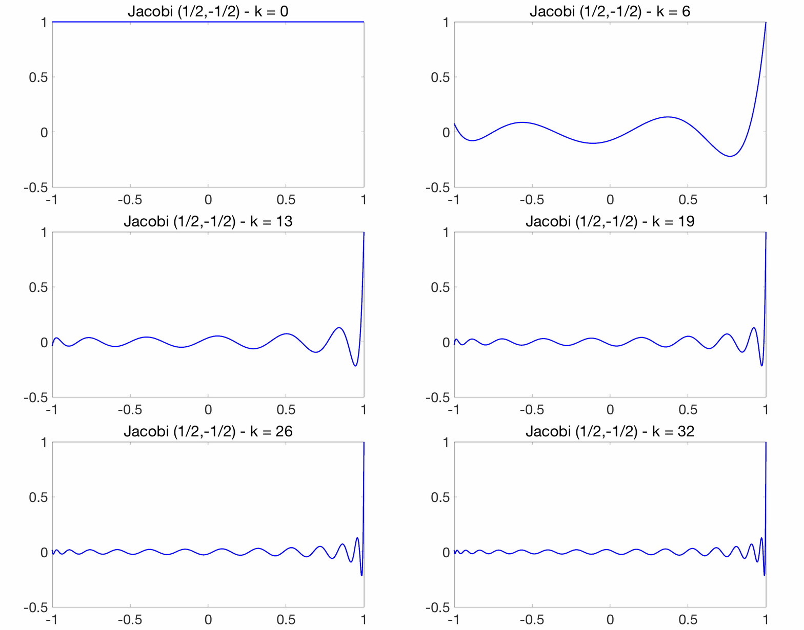
The class of Jacobi polynomials includes many of other important polynomials, such as Chebyshev polynomials (\(\alpha = \beta = -1/2\)), Legendre polynomials (\(\alpha = \beta = 0\)) and Gegenbauer polynomials (\(\alpha = \beta = d-1/2\)). Here are plots below.

Jacobi acceleration
We can now apply the polynomial acceleration technique above to the Beta distribution, that is for \(\displaystyle d\sigma(x) = \frac{1}{2^{\alpha+\beta+1} } \frac{\Gamma(\alpha+\beta +2)}{\Gamma(\alpha+1) \Gamma(\beta +1)} ( 1 -x )^\alpha (1+x)^\beta dx\), we have:
- Regular recursion error (no acceleration): the error \(e(X^k) = \displaystyle \int_{-1}^1 \lambda^{2k} d\sigma(\lambda)\) is asymptotically equivalent to \(\displaystyle \frac{C_{\alpha,\beta}}{k^{\alpha+1}}+\frac{C_{\beta,\alpha}}{k^{\beta+1}}\), for some constants \(C_{\alpha,\beta}\) (see details at the end of the post). Before acceleration, there is thus an equivalent impact of the spectrum around \(-1\) and \(1\).
- Jacobi acceleration error: as shown at the end of the post, the error \(e(P_k)\) is equivalent to \(\displaystyle \frac{E_{\alpha,\beta}}{k^{2\alpha+2}} \) for some constant \(E_{\alpha,\beta}\).
What’s happening around \(-1\) and \(1\) is important, and particular the behavior around 1, and we thus see that \(\beta\) is less important for the accelerated version (in fact, using \(\beta=0\) to construct the Jacobi polynomial, as done in [4], leads to a similar acceleration). In particular, when considering distributions where \(\beta = \alpha\), then we see that Jacobi acceleration transforms a rate proportional to \(1/k^{\alpha+1}\) to a rate proportional to \(1/k^{2\alpha+2}\).
The final recursion is then equal to (see detailed computations at the end of the post): $$ y_{k+1} = \frac{(2k\!+\!\alpha\!+\!\beta\!+\!2) }{2(k\!+\!2\!+\!\alpha\!+\!\beta)(k\!+\!\alpha\!+\!2) } \big[ (2k\!+\!3\!+\!\alpha\!+\!\beta) (Ay_k-b) + \frac{ (\alpha\!+\!1)^2\! -\! \beta^2 }{ 2k \!+\! 1\!+\!\alpha\!+\!\beta } y_k \Big] \ \ \ \ \ \ \ \ \ \ \ \ \ \ \ $$ $$\ \ \ \ \ \ \ \ \ \ \ \ \ \ \ \ \ \ \ \ \ \ \ \ \ \ \ \ \ \ \ \ \ \ \ \ \ \ \ \ \ \ \ – \frac{ (k+\beta)(2k +3+\alpha+\beta) }{ (k+2+\alpha+\beta) (2k + 1+\alpha+\beta )} \frac{ k }{ k+\alpha+2} y_{k-1}, $$ with initialization \(y_0=x_0\) and \(y_1 = \frac{\alpha+\beta+3}{2\alpha+4}(Ax_0 – b) + \frac{\alpha+1-\beta}{2\alpha+4}x_0\). For \(\alpha = \frac{d}{2}-1\) and \(\beta =0\), this exactly recovers the recursion from [4].
Application to gossip
Like in the previous post we consider the gossip problem. For large grid graphs, the gap is small, equivalent to \(\frac{1}{2d} \frac{1}{n^{2/d}}\) for the \(d\)-dimensional grid. The gap is tending to zero with \(n\), and using acceleration techniques for non-zero gaps, such as Chebyshev acceleration, is not efficient for the earlier iterations.
It turns out that for grid graphs, the spectral measure tends to a limit with behavior \((1-x^2)^{d/2-1}\) around \(-1\) and \(1\). This is formerly true for the grid graph, and the behavior around 1 (which is the one that matters for acceleration) is the same for a large class of graphs with an underlying geometric structure [4]. This thus corresponds to the Beta distribution of parameters \(\alpha = \beta = \frac{d}{2}-1\).
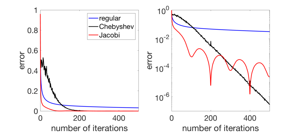
Below, I consider gossiping on a chain graph with \(n=200\) nodes, and compare regular gossip with Chebyshev acceleration and Jacobi acceleration. In early iterations, Jacobi acceleration is much better.

When looking at the convergence rate (plot below), for late iterations, the linear convergence of Chebyshev acceleration does take over; for a method that achieves the best of both world (good in early and late iterations), see [4, Section 7].

Similar plots may be made in two dimensions, gossiping a white noise signal, where the stationary behavior is observed much sooner for Jacobi acceleration. Here, Chebyshev acceleration performs worse than the regular iteration because the eigengap is very small (equal to \(6 \times 10^{-4}\)).

When gossiping a Dirac signal, we can also observe the spreading of information from the original position of the Dirac to the rest of the grid.

Conclusion
In this post, I tried to move from the worst-case analysis of spectral acceleration which typically focuses on largest and smallest eigenvalues of the involved contracting operators, closer to an average-case analysis that takes into account the whole spectrum. This led to acceleration by Jacobi polynomials rather than Chebyshev polynomials.
Beyond gossip. While I have focused primarily on applications to gossip where the spectral measure can be well approximated, this can be extended to other situations. For example, Fabian Pedregosa and Damien Scieur [5] recently considered an application of polynomial acceleration to gradient descent for least-squares regression with independent covariates, where the spectral measure of the covariance matrix tends to the famous Marchenko-Pastur distribution (which is close to the rescaled Beta distributions above).
Jacobi polynomials beyond acceleration. In this post, I focused only on the acceleration properties of Jacobi polynomials. There are many more interesting applications of these polynomials in machine learning and associated fields. For example, their role in spherical harmonics to provide an orthonormal basis of the square-integrable functions on the unit sphere in any dimension, is quite useful for the theoretical study of neural networks (see, e.g., [6] and references therein). I would typically say that this is a topic for another post, but this would be even more technical…
Next month, I will probably take a break in the polynomial magic series, and go back to less technical posts.
Acknowledgements. I would like to thank Raphaël Berthier for proofreading this blog post and making good clarifying suggestions.
References
[1] Bernd Fischer. Polynomial based iteration methods for symmetric linear systems. Springer, 1996.
[2] Gábor Szegő. Orthogonal Polynomials. American Mathematical Society, volume 23, 1939.
[3] Theodore Seio Chihara. An Introduction to Orthogonal Polynomials. Gordon and Breach, 1978.
[4] Raphaël Berthier, Francis Bach, Pierre Gaillard. Accelerated Gossip in Networks of Given Dimension using Jacobi Polynomial Iterations. To appear in SIAM Journal on Mathematics of Data Science, 2019.
[5] Fabian Pedregosa, Damien Scieur. Acceleration through Spectral Modeling. NeurIPS workshop “Beyond First Order Methods in ML”, 2019. [04/16/2020] Updated to: Average-case Acceleration Through Spectral Density Estimation, https://arxiv.org/pdf/2002.04756.pdf.
[6] Francis Bach. Breaking the Curse of Dimensionality with Convex Neural Networks. Journal of Machine Learning Research, 18(19):1-53, 2017.
Detailed computations
Kernel polynomial as orthogonal polynomial. We consider a series \((R_k)\) of orthogonal polynomials for the measure \((1-\lambda) d\sigma(\lambda)\). Assuming that \(R_k \neq 0\) (see proof in [4, Appendix D]), then we show that the polynomial \(\frac{R_k(X)}{R_k(1)}\) is the optimal polynomial of degree \(k\) minimizing \(\int_{-1}^1 P^2(\lambda) d\sigma(\lambda)\) such that \(P(1)=1\). Indeed, taking any polynomial \(P\) of degree \(k\) and such that \(P(1)=1\), the polynomial \(P(X) \, – \frac{R_k(X)}{R_k(1)}\) vanishes at \(1\) and can thus be written as \(A(X)(X-1)\) with \(A(X)\) of degree equal or less than \(k-1\). Then we have: $$\! \int_{-1}^1 \! \! P(\lambda)^2 d\lambda = \! \int_{-1}^1\!\! \frac{R_k(\lambda)^2}{R_k(1)^2}d\sigma(\lambda) + 2 \! \int_{-1}^1 \!\! \frac{R_k(\lambda)}{R_k(1)} A(\lambda)(\lambda-1)d\sigma(\lambda)+ \! \int_{-1}^1 \!\! \! A(\lambda)^2(\lambda-1)^2 d\sigma(\lambda).$$ The second term in the right hand side is equal to zero by orthogonality of \((R_k)\), and the third term is non-negative. Therefore, we must have \(\displaystyle \! \int_{-1}^1 \! \! P(\lambda)^2 d\lambda \geq \! \int_{-1}^1\!\! \frac{R_k(\lambda)^2}{R_k(1)^2}d\sigma(\lambda)\), which shows optimality.
Jacobi recursion. Given the original recursion \(x_{k+1} = A x_k – b\), we consider \(y_k = \frac{Q_k(A) ( x_0 – x_\ast)}{Q_k(1)} + x_\ast\), where \(Q_k = J_k^{(\alpha+1,\beta)}\). We get: $$ y_{k+1} = \frac{(a_k^{(\alpha+1,\beta)} A + b_k^{(\alpha+1,\beta)})Q_{k}(A)( x_0 – x_\ast) – c_k^{(\alpha+1,\beta)} Q_{k-1}(A) ( x_0 – x_\ast)}{Q_{k+1}(1)} + x_\ast.$$ This leads to $$ y_{k+1} = \frac{(a_k^{(\alpha+1,\beta)} A + b_k^{(\alpha+1,\beta)})Q_{k}(1) (y_k – x_\ast) – c_k^{(\alpha+1,\beta)} Q_{k-1}(1) ( y_{k-1} – x_\ast)}{Q_{k+1}(1)} + x_\ast.$$ Removing all terms in \(x_\ast\) (which have to cancel), we get: $$ y_{k+1} = a_k^{(\alpha+1,\beta)} \frac{Q_{k}(1)}{Q_{k+1}(1)}(Ay_k-b) + \tilde{b}_k^{(\alpha+1,\beta)} \frac{Q_{k}(1)}{Q_{k+1}(1)}y_k – c_k^{(\alpha+1,\beta)} \frac{Q_{k-1}(1)}{Q_{k+1}(1)}y_{k-1}. $$ Using the explicit formula for \(Q_{k}(1)\), we get after some calculations: $$ y_{k+1} = \frac{(2k\!+\!\alpha\!+\!\beta\!+\!2) }{2(k\!+\!2\!+\!\alpha\!+\!\beta)(k\!+\!\alpha\!+\!2) } \big[ (2k\!+\!3\!+\!\alpha\!+\!\beta) (Ay_k-b) + \frac{ (\alpha\!+\!1)^2\! -\! \beta^2 }{ 2k \!+\! 1\!+\!\alpha\!+\!\beta } y_k \Big] \ \ \ \ \ \ \ \ \ \ \ \ \ \ \ $$ $$\ \ \ \ \ \ \ \ \ \ \ \ \ \ \ \ \ \ \ \ \ \ \ \ \ \ \ \ \ \ \ \ \ \ \ \ \ \ \ \ \ \ \ – \frac{ (k+\beta)(2k +3+\alpha+\beta) }{ (k+2+\alpha+\beta) (2k + 1+\alpha+\beta )} \frac{ k }{ k+\alpha+2} y_{k-1}, $$ with initialization \(y_0 = x_0\) and \(y_1 = \frac{\alpha+\beta+3}{2\alpha+4}(Ax_0 – b) + \frac{\alpha+1-\beta}{2\alpha+4}x_0\).
Equivalents of performance. We first provide an equivalent of $$ \int_{-1}^1 \lambda^{2k} d\sigma(\lambda) = \frac{1}{2^{\alpha+\beta+1} } \frac{\Gamma(\alpha+\beta +2)}{\Gamma(\alpha+1) \Gamma(\beta +1)}\int_{-1}^1 \! x^{2k} (1-x)^\alpha(1+x)^\beta dx.$$ By splitting the sum in two, this is equivalent to $$ \frac{1}{2^{\alpha+\beta+1} } \frac{\Gamma(\alpha+\beta +2)}{\Gamma(\alpha+1) \Gamma(\beta +1)}\Big\{ 2^\beta\!\! \int_{0}^1 \! x^{2k} (1-x)^\alpha dx + 2^\alpha \!\! \int_{0}^1 \! x^{2k}(1-x)^\beta dx \Big\},$$ leading to, using the normalizing factor of the Beta distribution, $$\frac{1}{2^{\alpha+\beta+1} } \frac{\Gamma(\alpha+\beta +2)}{\Gamma(\alpha+1) \Gamma(\beta +1)} \Big\{ 2^\beta\frac{\Gamma(\alpha+1)\Gamma(2k+1)}{\Gamma(\alpha+2k+2)} +2^\alpha\frac{\Gamma(\beta+1)\Gamma(2k+1)}{\Gamma(\beta+2k+2)} \Big\}, $$ and finally to $$ \displaystyle \frac{1}{2^{\alpha+\beta+1} } \frac{\Gamma(\alpha+\beta +2)}{\Gamma(\alpha+1) \Gamma(\beta +1)} \Big\{ 2^\beta\frac{\Gamma(\alpha+1) }{ (2k/e)^{\alpha+1} } +2^\alpha\frac{\Gamma(\beta+1) }{ (2k/e)^{\beta+1} } \Big\} ,$$ which is indeed of the form \(\displaystyle \frac{C_{\alpha,\beta}}{k^{\alpha+1}}+\frac{C_{\beta,\alpha}}{k^{\beta+1}}\).
In order to estimate \(e(P_k)\), since \(P_k(X) = \sum_{i=0}^k \frac{1}{\alpha_i} Q_i(1) Q_i(X)\), we first need an equivalent of the term \(\displaystyle \frac{Q_i(1)^2}{\alpha_i^2} \sim \frac{(i/e)^{2\alpha}}{\Gamma(\alpha+1)^2} \Big( \frac{\Gamma(\alpha+\beta +2)}{\Gamma(\alpha+1) \Gamma(\beta +1) }\frac{1}{2i}\Big)^{-1} \sim E_{\alpha,\beta}’ i^{2\alpha+1}\), for some \(E_{\alpha,\beta}’\), leading to an error of the form \(e(P_k) \displaystyle \sim \frac{1}{ E_{\alpha,\beta}’ \sum_{i=0}^k i^{2\alpha+1}} \sim\frac{2\alpha+2}{ E_{\alpha,\beta}’} \frac{1}{k^{2\alpha+2}} \), which is of the desired form.
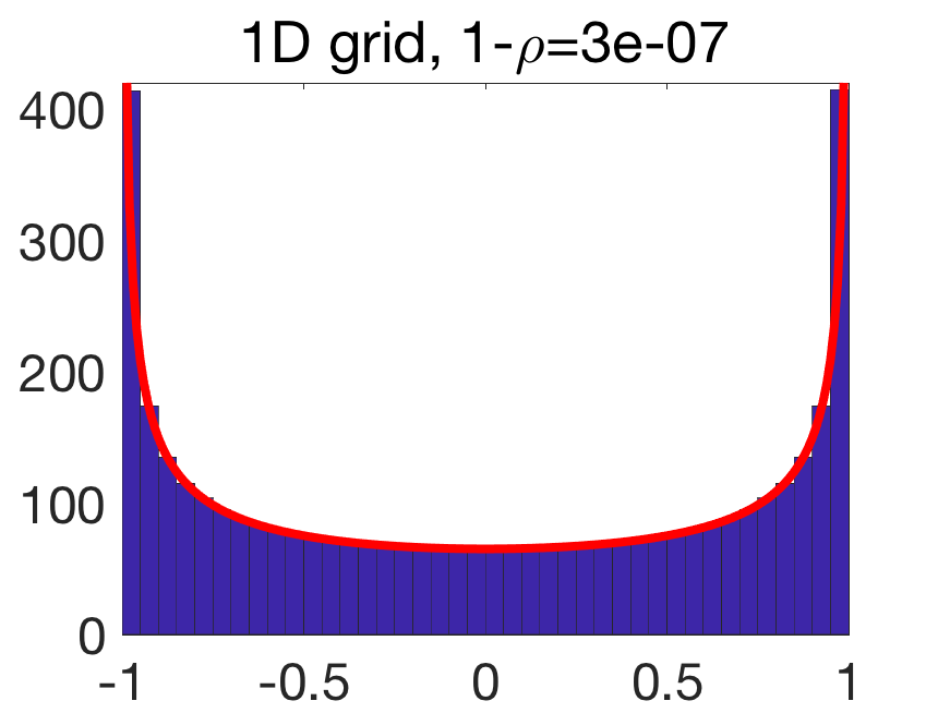
Spectral density of a grid. As seen at the far end of the previous blog post, the eigenvalues of \(A\) for the grid in one-dimension, with \(m=n\), is (up to negligible corrections) \(– \cos \frac{k\pi}{m}\) for \(k =1,\dots,m\). This leads to a limiting spectral measure as \(– \cos \theta\) for \(\theta\) uniformly distributed on \([0,\pi]\). This leads to a spectral density \(\frac{1}{\pi}\frac{1}{\sqrt{1-\lambda^2}}\) supported on \([-1,1]\). In the plot below, we see that the histogram of eigenvalues for a finite \(m\) matches empirically this density.

For a \(d\)-dimensional grid, with \(n = m^d\), the spectral density is the one of \(\frac{1}{d} (X_1+\cdots X_d)\) for \(X_i\) independent and distributed as \(\frac{1}{\pi}\frac{1}{\sqrt{1-\lambda^2}} d\lambda\) on \([-1,1]\), for each \(i=1,\dots,d\). This leads to a convolution power of the density above, rescaled to have support in \([-1,1]\). This can be shown to lead to behavior as \((1-\lambda^2)^{d/2-1}\) around \(1\) and \(-1\) (see [4, Prop. 5.2]).