The quest for adaptivity

Most machine learning classes and textbooks mention that there is no universal supervised learning algorithm that can do reasonably well on all learning problems. Indeed, a series of “no free lunch theorems” state that even in a simple input space, for any learning algorithm, there always exists a bad conditional distribution of outputs given inputs where this algorithm performs arbitrarily bad.

For example, from the classic book of Luc Devroye, László Györfi, and Gábor Lugosi [1, Theorem 7.2 and its extensions], for inputs uniformly distributed in \([0,1]\), for any decreasing sequence \((\varepsilon_n)_{n \geqslant 0}\) which is less than 1/16, for any learning algorithm (which takes pairs of observations and outputs a prediction function), there exists a conditional distribution on \(\{-1,1\}\) for which the expected risk of the classifier learned from \(n\) independent and identically distributed observations of (input,output) pairs is greater than \(\varepsilon_n\) for all \(n \geqslant 1\), while the best possible expected error rate is zero.

Such theorems do not imply that all learning methods are equally bad, but rather that all learning methods will suffer from some weaknessess. Throughout this blog we will try to better understand the weaknessess and strengths of popular methods through learning theory.

The key is to control the potential weaknesses of a learning method by making sure that in “favorable” scenarios, it leads to strong guarantees. When taking the simplest example of vectorial inputs in \(\mathbb{R}^d\), we can construct model classes of increasing complexity for which we can start to draw useful comparisons between learning methods.

Several aspects of the joint distribution of (input,output) \((X,Y)\) make the problem easy or hard. For concreteness and simplicity, I will focus on regression problems where the output space is \(\mathcal{Y} = \mathbb{R}\) and with the square loss, so that the optimal function, the “target” function, is \(f^\ast(x) = \mathbb{E}(Y|X=x)\). But much of the discussion extends to classification or even more complex outputs (see, e.g., [1]).

Curse of dimensionality. In the context of vectorial inputs, the slowness of universal learning algorithms can be characterized more precisely, and leads to the classical curse of dimensionality. Only assuming that the optimal target function is Lipschitz-continuous, that is, for all \(x,x’\), \(| f^\ast(x)-f^\ast(x’)| \leqslant L \| x – x’\|\) (for any arbitrary norm on \(\mathbb{R}^d\)), the optimal excess risk of a prediction function \(\hat{f}\) obtained from \(n\) observations, that is, the expected squared difference between \(f^\ast(x)\) and \(\hat{f}(x)\) cannot be less than a constant times \(n^{-2/(d+2)}\), that is, in order for this rate to be smaller than some \(\varepsilon <1 \), we need \(n\) to be larger than \(\displaystyle ( {1}/{\varepsilon} )^{d/2+1}\), with thus an exponential dependence in \(d\) (see [2]).

In other words, exponentially many observations are needed for a reasonable performance on all problems with a minimal set of assumptions (here Lipschitz-continuity), and this bad behavior is unavoidable unless extra assumptions are added, which we now describe.

Support, smoothness and latent variables

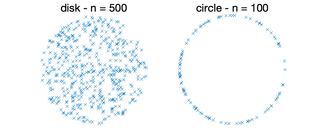
Low-dimensional support. If the data occupy only a \(r\)-dimensional subspace of \(\mathbb{R}^d\), with \(r \leqslant d\) (and typically much smaller), then one should expect a better convergence rate. This also extends to data supported on a (smooth) manifold, as illustrated below. Note that this assumption does not concern the outputs, and can reasonably be checked given the data by performing principal component analysis or some form of manifold learning. Essentially, in terms of convergence rates, \(d\) is replaced by \(r\). This is obvious if the learning algorithm has access to the \(r\)-dimensional representation, and it requires more work if not.

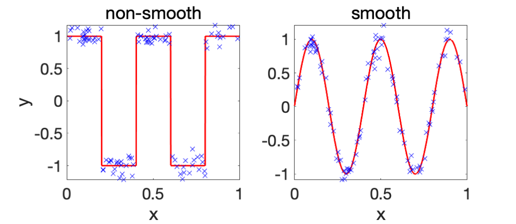
Smoothness of the target function. This is done by assuming some bounded derivatives for the target function \(f^\ast\). With bounded \(s\)-th order derivatives, we could expect that the problem is easier (note that Lipschitz-continuity corresponds to \(s=1\)). This is illustrated below with one-dimensional inputs. Essentially, in terms of rates, \(d\) is replaced by \(d/s\) [2, Theorem 3.2]. Therefore, when the smoothness order \(s\) is of order \(d\), the dependence in the dimension disappears.

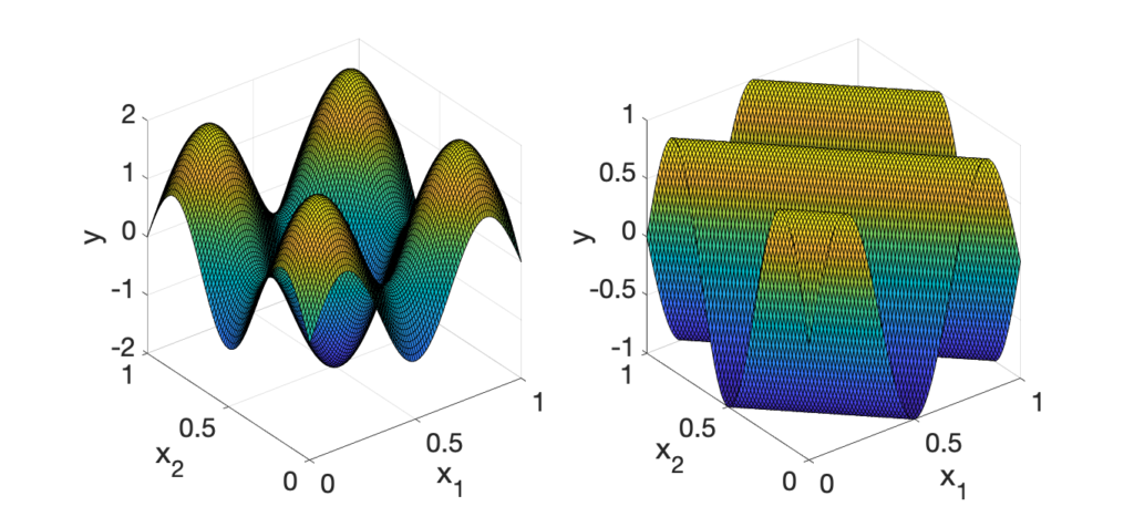
Latent variables. If we assume that the target function depends only on a \(r\)-dimensional linear projection of the input, then we should expect a better complexity. The most classical example is the dependence on a subset of the \(d\) original variables. Essentially, in terms of rates, \(d\) is replaced by \(r\). This is obvious when the latent variables are known (as we can replace input data by the \(r\) latent variables), totally not otherwise, as this requires some form of adaptivity (see below).

Need for adaptivity. We typically don’t know in advance if these properties are satisfied or not, as some are easily testable (support of distribution) without knowing the target function \(f^\ast\), while others are not.

The goal is to have a single method that can adapt to all of these situations (which are non-exclusive). That is, if the problem has any of these reasons to be easy, will the learning method benefit from it? Typically, most learning methods have at least one hyperparameter controlling overfitting (e.g., a regularization parameter), and the precise value of this hyperparameter will depend on the difficulty of the problem, and we will assume that we have a reasonable way to estimate this hyperparameter (e.g., cross-validation). A method is then said adaptive if with a well chosen value of the hyperparameter, we get the optimal (or close to optimal) rate of estimation that benefits from the extra assumption.

Quest for adaptivity: who wins? Among classical learning techniques, which ones are adaptive to which properties? In short, barring computational and optimization issues: $$\mbox{ local averaging } < \mbox{ positive definite kernels } < \mbox{ neural networks }.$$ Every time, the next method in the list gains adaptivity to support, smoothness and then latent variables. Note however that optimization for neural networks is more delicate (see below).

Let’s now briefly look at these methods one by one. I will assume basic knowledge of these, for more details see [4, 5] or my new book in preparation.

Local averaging

The earliest and simplest learning methods that could adapt to any target functions were local averaging methods aiming at approximating directly the conditional expectation \(f^\ast(x) = \mathbb{E}(Y|X=x)\), with the most classical examples being k-nearest neighbors and Nadaraya-Watson estimators.

These methods are naturally adaptive to having a reduced support for inputs. Indeed, in the simplest case of a distribution supported in a low-dimensional subspace, the global metric is equivalent to a local metric on the support, without any need to explicitly know the subspace, a situation which extends to smooth manifolds. In order to be adaptive, the hyperparameter has to depend on the dimension \(r\) of the manifold, e.g., for \(k\)-nearest-neighbors, \(k\) has to be taken proportional to \(n^{2/(2+r)}\) (see [3]).

However, there is no adaptivity to the smoothness of the target function or to potential latent variables unless dedicated algorithms are used such as local regression. Kernel methods and neural networks lead to such adaptivity.

From kernels to neural networks

We consider prediction functions of the form $$f(x) = \sum_{j=1}^m a_j ( b_j^\top x )_+,$$ which is the traditional single hidden layer fully connected neural network with ReLU activation functions (a constant term can be added to the linear term within the ReLU by simply appending \(1\) to \(x\), please do not call these terms “biases” as this has another meaning in statistics).

The vector \(a \in \mathbb{R}^m\) represents output weights, while the matrix \(b \in \mathbb{R}^{m \times d}\) represents input weights.

Empirical risk minimization (ERM). We assume given \(n\) i.i.d. observations \((x_1,y_1),\dots,(x_n,y_n) \in \mathbb{R}^d \times \mathbb{R}\), and we will fit models by minimizing the \(\ell_2\)-regularized empirical risk (you can call it “weight decay” but it already has a better name in machine learning and statistics). That is, we minimize $$R(a,b) = \frac{1}{2n} \sum_{i=1}^n \Big( y_i \, – \sum_{j=1}^m a_j ( b_j^\top x_i )_+ \Big) ^2 + \frac{\lambda}{2} \sum_{j=1}^m \Big\{ a_j^2 + \| b_j\|_2^2 \Big\},$$ where \(\lambda > 0\) is a regularization parameter.

Overparametrization. We will consider the limit of large number \(m\) of hidden neurons. Depending whether we optimize over both input weights \(b\) and output weights \(a\), or simply output weights (with then a proper initialization of the input weights), we get different behaviors.

Kernel regime

We assume that the input weights \(b_j \in \mathbb{R}^d\) are sampled uniformly from the Euclidean sphere of radius \(1 / \sqrt{m}\), and that we only optimize over the output weights \(a_j, j = 1,\dots,m\). This is exactly a ridge regression problem (square loss and squared Euclidean penalty), for which the theory of positive definite kernels applies and will lead to an interesting behavior for infinite \(m\) [7, 8]. That is, the solution can be obtained by using the kernel function \(\hat{k}\) defined as $$\hat{k}(x,x’) = \sum_{j=1}^m ( b_j^\top x )_+( b_j^\top x’ )_+,$$ and looking for prediction functions of the form $$f(x) = \sum_{i=1}^n \alpha_i \hat{k}(x,x_i).$$ See, e.g., [6] for details. In particular, as long as \(\hat{k}(x,x’)\) can be computed efficiently, the complexity of solving the ERM problem is independent of the number of neurons \(m\). We will now discuss in further detail the over-parameterized case where \(m=\infty\).

When \(m\) tends to infinity, If the input weights are fixed and initialized randomly from the \(\ell_2\)-sphere of radius \(1/\sqrt{m}\), then by the law of large numbers, \(\hat{k}(x,x’)\) tends to $$k(x,x’) = \mathbb{E}_{b \sim {\rm uniform} (\mathbb{S}^{d-1}) } (b^\top x )_+ (b^\top x’)_+,$$ where \(\mathbb{S}^{d-1}\) is the unit \(\ell_2\)-sphere in \(d\) dimensions. This kernel has a closed form and happens to be equal to (see [9]) $$ \frac{1}{2\pi d} \|x\|_2 \| x’\|_2 \big[ ( \pi \, – \varphi) \cos \varphi + \sin \varphi \big],$$ where \(\cos \varphi = \frac{ x^\top x’ }{{ \|x\|_2 } { \| x’\|_2 } }\). It can also be seen (see, e.g., [10] for details) as using predictors of the form $$f(x) = \int_{\mathbb{S}^{d-1}} ( b^\top x)_+ d \mu(b),$$ for some measure \(\mu\) on \(\mathbb{S}^{d-1}\), with the penalty $$\frac{\lambda}{2} \int_{\mathbb{S}^{d-1}} \big| \frac{d\mu}{d\tau}(b) \big|^2 d\tau(b),$$ for the uniform probability measure \(d\tau\) on the hypersphere \(\mathbb{S}^{d-1}\). This representation will be useful for the comparison with neural networks.

Note that here we use random features in a different way from their common use [8], where the kernel \(k\) comes first and is approximated by \(\hat{k}\) to obtain fast algorithms, typically with \(m < n\). Here we start from \(\hat{k}\) and find the limiting \(k\) to understand the behavior of overparameterization. The resulting function space is a (Sobolev) space of functions on the sphere with all \(s\)-th order derivatives which are square-integrable, with \(s = d/2+3/2\) [10].

Finally, the number of neurons \(m\) needed to reach the kernel regime is well understood, at least in simple situations [15, 16].

We can now look at the various forms of adaptivity of kernel methods based on Sobolev spaces.

Adaptivity to reduced support. Like model averaging techniques, adaptivity to input data supported on a subspace is rather straightforward, and it extends to smooth manifolds (see, e.g., [12] for a proof for the Gaussian kernel).

Adaptive to smoothness. A key attractive feature of kernel methods is that they can circumvent the curse of dimensionality for smooth target functions, and, by simply ajusting the regularization parameter \(\lambda\), ridge regression will typically adapt to the smoothness of the target function, and thus benefit from easy problems.

The simplest instance is when the target function is within the space of functions defined above, where we immediately get estimation rates which are independent of dimension (at least in the exponent). This however requires at least \(s>d/2\) derivatives (because Sobolev spaces are reproducing kernel Hilbert spaces (RKHS) only in this situation), but the adaptivity extends to functions outside of the RKHS (see, e.g., [11]).

Adaptivity to linear latent variables. Unfortunately, kernel methods are not adaptive even to basic linear structures. That is, if \(f^\ast\) depends only on the first component of \(x\), then ridge regression, if not modified, will not take advantage of it. In the context of neural networks, one striking example is that a single neuron \(x \mapsto (b^\top x)_+\) does not belong to the RKHS, and leads to bad estimation rates (see, e.g., [10, 13]).

Before looking at some experiments, let’s look at some optimization considerations, that will be important later for neural networks.

Avoiding overparameterized neuron representations. In the kernel regime, optimizing directly the cost function with \(m\) neurons by gradient descent is problematic for two reasons when \(m\) is large:

• The optimization problem, although convex, is severely ill-conditioned as can be seen from the spectrum of the covariance matrix of the feature vector, with the \(i\)-th eigenvalue equivalent to \(i^{-1-3/d}\) for the uniform input distribution (see [14, Section 2.3]). Therefore, (stochastic) gradient descent will take a lot of time to converge.
• We can use kernels directly (for \(m = +\infty\)) to avoid using \(m\) very large (which would be useless in practice). The running-time complexity is then of the order \(O(n^2)\) if done naively, with lots of ways to go below \(O(n^2)\), such as column sampling (see a nice analysis in [15]).

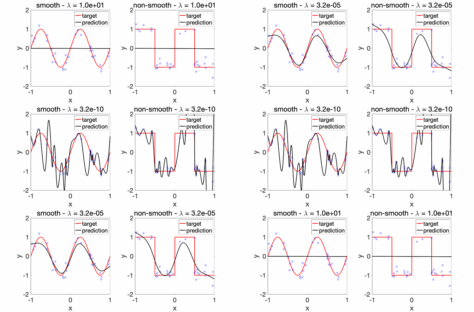
Experiments. We first consider a very simple one-dimensional example, where we look at how the estimation with the kernel function \(k\) varies as a function of the hyperparameter \(\lambda\), from underfitting to overfitting. We can observe that all learned functions are smooth, as expected.

We can now compare the convergence rates for the excess risk (expected squared distance beween \(f\) and \(f^\ast\)). We can see that the rates are better for smooth functions, and with the proper choice of regularization parameter, the kernel method adapts to it.

Neural networks

We can now optimize over all weights, output \(a\) and input \(b\). Four natural questions come to mind:

1. Where does it converge to when the number \(m\) of hidden neurons tends to infinity?
2. What are the adaptivity properties of the resulting predictor?
3. How big \(m\) needs to be to achieve the infinite width behavior?
4. Can we actually solve the non-convex optimization problem?

Overparameterization limit (feature learning regime). When optimizing over both sets of weights, we can first note that the prediction function is invariant by the change of variable $$ a_j \leftarrow \mu_j a_j \ , \ \ b_j \leftarrow \mu_j^{-1} b_j.$$ Then by optimizing over \(\mu_j\) which is only involved in the penalty term \(\frac{\lambda}{2} \big( a_j^2 + \|b_j\|_2^2 \big)\), we get \(\mu_j^\ast = a_j^{-1/2} \| b_j \|_2^{1/2}\), and the penalty \(\lambda |a_j| \| b_j\|_2\). We thus get the equivalent optimization problem of minimizing $$\tilde{R}(a,b) = \frac{1}{2n} \sum_{i=1}^n \Big( y_i \, – \sum_{j=1}^m a_j ( b_j^\top x_i )_+ \Big) ^2 + {\lambda} \sum_{j=1}^m |a_j| \| b_j\|_2 .$$ By restricting the \(b_j\) on the unit sphere (which is OK because by optimizing over \(\mu_j\) we become scale-invariant), we can write $$\sum_{j=1}^m a_j ( b_j^\top x_i )_+ = \int_{\mathbb{S}^{d-1}} (b^\top x)_+ d\mu(b), $$ for $$ \mu = \sum_{j=1}^m a_j \delta_{b_j}$$ a weighted sum of Diracs, and \(\sum_{j=1}^m |a_j| \| b_j\|_2 = \int_{\mathbb{S}^{d-1}} \! | d\mu(b)|\) the total variation of \(\mu\). Thus, letting \(m\) go to infinity, the infinite sums become integrals of general measures, and we end up considering the set of functions that can be written as (see [10] and the many references therein for details): $$f(x) = \int_{\mathbb{S}^{d-1}} ( b^\top x)_+ d \mu(b),$$ with the penalty $$\lambda \int_{\mathbb{S}^{d-1}} \! | d\mu(b)|.$$ It has an \(\ell_1\)-norm flavor (as opposed to the \(\ell_2\)-norm for kernels), and leads to further adaptivity, if optimization problems are resolved (which is itself not easy in polynomial time, see below).

The minimal number of neurons to achieve the limiting behavior in terms of predictive performance (assuming optimization problems are resolved) can also be characterized, and grows exponentially in dimension without strong assumptions like the ones made in this blog post (see [10]). We will now study the adaptivity properties of using the function space above.

Adaptive to low-dimensional support and smoothness. It turns out that the adaptivity properties of kernel methods are preserved, both with respect to the support and the smoothness of the target function (see, e.g., [17, 10]). However, neural networks can do better!

Adaptive to linear substructures for one hidden layer. Given that the training of neural networks involves finding the best possible input weights, which are involved in the first linear layer, it is no surprise that we obtain adaptivity to linear latent variables. That is, if we can write \(f^\ast(x) = g(c_1^\top x, \dots, c_r^\top x)\) for some function \(g: \mathbb{R}^r \to \mathbb{R}\), then the vectors \(c_j\)’s will be essentially estimated among the \(b_j\)’s by the optimization algorithm. Therefore, when using the \(\ell_1\)-based function space, the convergence rate in the excess risk will depend on \(r\) and not \(d\) in the exponent [10, 13]. In particular, neural networks can perform non-linear variable selection (while the Lasso only performs linear variable selection). See a nice experiment in [13] for binary classification.

One could imagine that with more hidden layers, this extends to non-linear smooth projections of the data, that is, to cases where we assume that \(f^\ast(x) = g(h(x))\) where \(h: \mathbb{R}^d \to \mathbb{R}^r\) is a smooth function.

Thus, we obtain a stronger adaptivity for infinite \(m\) and the good choice of regularization parameter \(\lambda\). We could then try to reproduce for neural networks the figures obtained for kernel methods with varying \(\lambda\). Unfortunately, this is where non-convex optimization will make everything harder.

Overfitting with a single hidden layer is hard!

Global convergence of gradient flow for infinite width. The traditional algorithm to minimize the empirical risk is gradient descent and its stochastic extensions. In this blog post, we consider gradient descent with small step-sizes, which can be approximated by a gradient flow (as explained in last June blog post). All parameters are randomly initialized, and we consider \(b_j\) uniformly distributed on the sphere of radius \(1/\sqrt{m}\), and \(a_j\) uniformly distributed in \(\{-1/\sqrt{m},1/\sqrt{m}\}\) (this is essentially equivalent to the traditional “Glorot” initialization [18]).

This corresponds to the “mean-field” scaling of initialization where neurons from both layers move (see more details in last July blog post for other scalings). As shown in a joint work with Lénaïc Chizat [19] and explained in last June blog post, when \(m\) tends to infinity, then the gradient flow can only converge to the global minimum of the objective function, which is a non-trivial result because the cost function is not convex in \((a,b)\).

Apparent good properties for small \(m\). A key property which is not yet well understood is that the global convergence behavior can be observed for \(m\) relatively small. For example, considering the one-dimensional regression example below, where the target function is the combination of 5 hidden neurons, with \(m=32\) hidden neurons, it is already possible to learn a good function with high probability (this would not be the case with \(m=5\)).

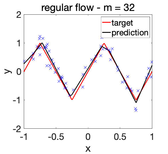
One extra benefit here is that no regularization (e.g., no penalty) seems needed to obtain this good behavior. Therefore it seems that we get the best of both worlds: reasonably small \(m\) (so not too costly algorithmically), and no need to regularize.

However, like in any situation where overfitting is not observed, there is the possibility of underfitting. To study this, let us consider a noiseless problem where \(y\) is a deterministic function of \(x\), and with a sligthly more complicated target function, which now requires 9 hidden neurons.

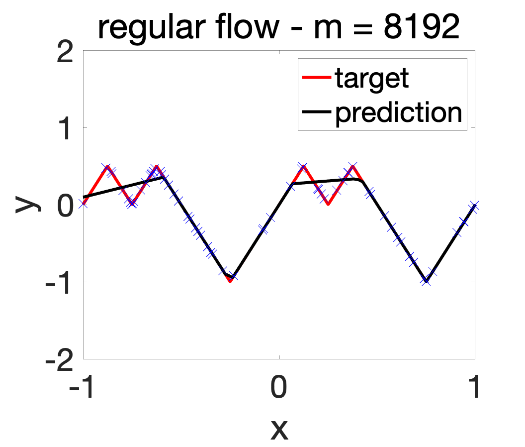
Even with \(m = 8192\) hidden neurons, the resulting function is not able to fit the data, which is one extreme form of simplicity bias [21]. There is thus strong underfitting with a single hidden layer (the situation seems to be different with deeper networks). How can this be alleviated?

Kernel learning to the rescue

A simple way to avoid the underfitting phenomenon above (but potentially get overfitting, see below) is to minimize the cost \(R(a,b)\) by leveraging a convex sub-problem, as done in the glorious days of kernel methods.

In the cost function $$R(a,b) = \frac{1}{2n} \sum_{i=1}^n \Big( y_i \, – \sum_{j=1}^m a_j ( b_j^\top x_i )_+ \Big) ^2 + \frac{\lambda}{2} \sum_{j=1}^m \Big\{ a_j^2 + \| b_j\|_2^2 \Big\},$$ the problem is convex with respect to all \((a_j)\)’s; moreover, it is a least-squares problems which can be solved in closed form by matrix inversion (with algorithms that are much more robust to ill-conditioning than gradient descent).

Then, if we denote by \(\Phi(b) \in \mathbb{R}^{n \times m}\) the matrix with elements \((b_j^\top x_i)_+\), the cost function can be written as a function of \(a \in \mathbb{R}^m\) as $$R(a,b) = \frac{1}{2n} \| y \, – \Phi(b) a \|_2^2 +\frac{\lambda}{2}\| a\|_2^2 + \frac{\lambda}{2} \sum_{j=1}^m \| b_j\|_2^2.$$ It can be minimized in closed form as $$ a = ( \Phi(b)^\top \Phi(b) + n \lambda I)^{-1} \Phi(b)^\top y = \Phi(b)^\top ( \Phi(b)\Phi(b)^\top + n \lambda I)^{-1} y,$$ where the matrix inversion lemma has been used. This leads to: $$S(b) = \inf_{a \in \mathbb{R}^m} R(a,b) = \frac{\lambda}{2} y^\top ( \Phi(b)\Phi(b)^\top + n \lambda I)^{-1} y + \frac{\lambda}{2} \sum_{j=1}^m \| b_j\|_2^2.$$ The matrix \(\Phi(b)\Phi(b)^\top \in \mathbb{R}^{n \times n}\) is the traditional kernel matrix of the associated non-linear features. The resulting optimization problem is exactly one used in kernel learning [20].

Computing \(S(b)\) and its gradient with respect to \(b\) can be done in time \(O(n^2 m)\) when \(m\) is large. Since given the hidden neurons, we get the global optimum, we avoid the underfitting problem as well as the ill-conditioning issues.

When \(m\) tends to infinity, then the optimization problem fits our analysis in [19], that is, we can see the limiting flow as a Wasserstein gradient flow that can only converge to the global optimum of the associated cost function although the overall problem is not convex (as opposed to what happens in multiple kernel learning described in this older post). While there is currently no further quantitative theoretical evidence that a good optimization behavior can be reached for a smaller \(m\), it empirically solves the underfitting issue above, as shown below.

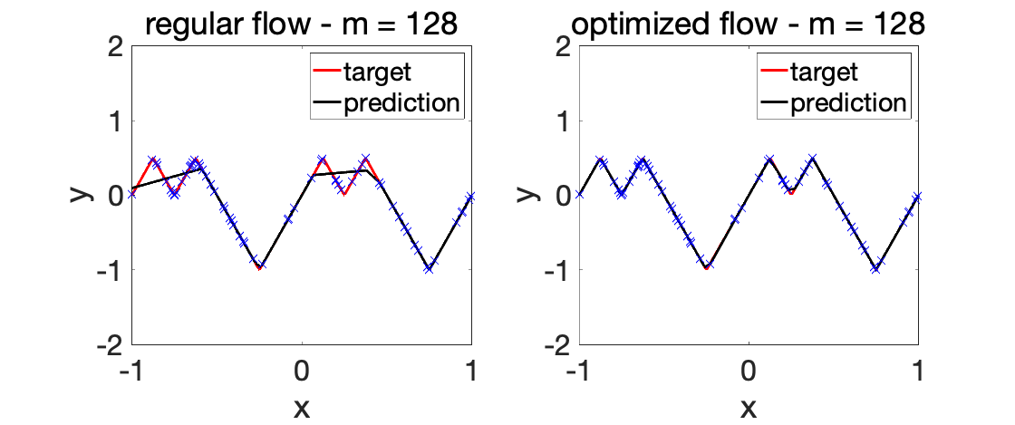
We can now perform experiments with varying \(\lambda\)’s.

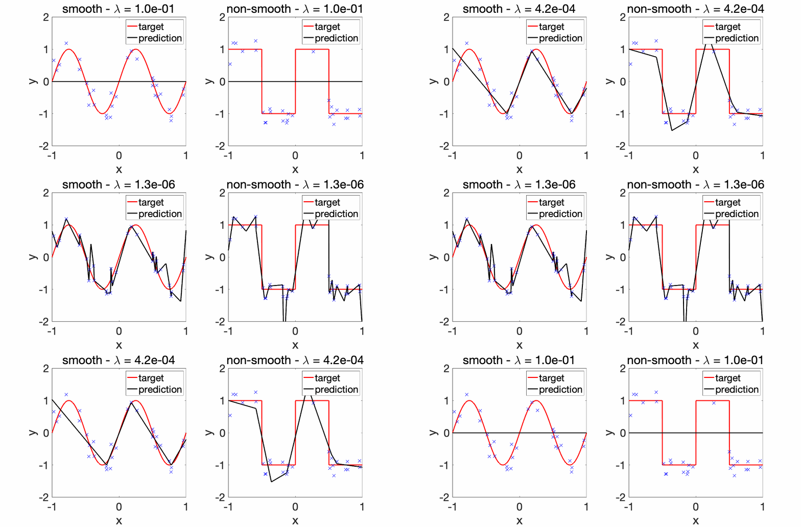
Experiments. The two plots below depict the learnt functions for a smooth and non-smooth objective as \(\lambda\) is varied, highlighting the importance of regularization.

We can now compare the convergence rates for the excess risk (expected squared distance beween \(f\) and \(f^\ast\)). We can see that the rates are better for smooth functions, and with the proper choice of regularization parameter, neural networks adapt to it. For adaptivity to linear latent variables, see [13].

Conclusion

As I tried to show in this blog post, adaptivity is a key driver of good predictive performance of learning methods. It turns out that for the three classes of methods I considered, the more complex algorithms led to more adaptivity: no optimization for local averaging, finite-dimensional convex optimization for kernel methods and then non-convex optimization for neural networks (or equivalently infinite-dimensional convex optimization).

While neural networks led to more adaptivity, they are still not totally well understood, in particular in terms of the various biases that their training implies, both for shallow and deep networks. This makes a lot of research directions to follow!

Acknowledgements. I would like to thank Lénaïc Chizat and Lawrence Stewart for proofreading this blog post and making good clarifying suggestions.

References

[1] Luc Devroye, László Györfi, and Gábor Lugosi. A Probabilistic Theory of Pattern Recognition,
volume 31. Springer Science & Business Media, 1996.
[2] László Györfi, Michael Kohler, Adam Krzyżak, Harro Walk. A Distribution-free Theory of Nonparametric Regression. New York : Springer, 2002.
[3] Samory Kpotufe. k-NN regression adapts to local intrinsic dimension. In Advances in Neural Information Processing Systems, 2011.
[4] Mehryar Mohri, Afshin Rostamizadeh, and Ameet Talwalkar. Foundations of Machine Learning. MIT Press, 2018.
[5] Shai Shalev-Shwartz and Shai Ben-David. Understanding Machine Learning: From Theory to Algorithms. Cambridge University Press, 2014.
[6] Bernhard Schölkopf and Alexander J. Smola. Learning with Kernels. MIT Press, 2001.
[7] Radford M. Neal. Bayesian Learning for Neural Networks. PhD thesis, University of Toronto, 1995.
[8] Ali Rahimi and Benjamin Recht. Random features for large-scale kernel machines. In Advances in Neural Information Processing Systems, 2008.
[9] Youngmin Cho and Lawrence K. Saul. Kernel methods for deep learning. In Advances in Neural Information Processing Systems, 2009.
[10] Francis Bach. Breaking the curse of dimensionality with convex neural networks. The Journal of Machine Learning Research, 18(1):629–681, 2017.
[11] Andreas Christmann, Ingo Steinwart. Support Vector Machines. Springer, 2008.
[12] Thomas Hamm, Ingo Steinwart. Adaptive Learning Rates for Support Vector Machines Working on Data with Low Intrinsic Dimension. Technical report, Arxiv 2003.06202, 2021.
[13] Lénaïc Chizat, Francis Bach. Implicit Bias of Gradient Descent for Wide Two-layer Neural Networks Trained with the Logistic Loss. Proceedings of the Conference on Learning Theory (COLT), 2020.
[14] Francis Bach. On the Equivalence between Kernel Quadrature Rules and Random Feature Expansions. Journal of Machine Learning Research, 18(19):1-38, 2017. 
[15] Alessandro Rudi, Raffaello Camoriano, and Lorenzo Rosasco. Less is more: Nyström computational regularization. In Advances in Neural Information Processing Systems, pages 1657–1665, 2015.
[16] Alessandro Rudi, Lorenzo Rosasco. Generalization properties of learning with random features. In Advances in Neural Information Processing Systems, 2017.
[17] Ryumei Nakada, Masaaki Imaizumi. Adaptive Approximation and Generalization of Deep Neural Network with Intrinsic Dimensionality. Journal of Machine Learning Research, 21(174):1−38, 2020.
[18] Xavier Glorot, Yoshua Bengio. Understanding the difficulty of training deep feedforward neural networks. Proceedings of the International Conference on Artificial Intelligence and Statistics, 2010.
[19] Lénaïc Chizat, Francis Bach. On the Global Convergence of Gradient Descent for Over-parameterized Models using Optimal Transport. Advances in Neural Information Processing Systems, 2018
[20] Olivier Chapelle, Vladimir Vapnik, Olivier Bousquet, Sayan Mukherjee. Choosing multiple parameters for support vector machines. Machine Learning, 46(1):131-159, 2002.
[21] Harshay Shah, Kaustav Tamuly, Aditi Raghunathan, Prateek Jain, Praneeth Netrapalli. The Pitfalls of Simplicity Bias in Neural Networks. In Advances in Neural Information Processing Systems, 2020.