It seemed a bit unfair to devote a blog to machine learning (ML) without talking about its current core algorithm: stochastic gradient descent (SGD). Indeed, SGD has become, year after year, the basic foundation of many algorithms used for large-scale ML problems. However, the history of stochastic approximation is much older than that of ML: its first study by Robbins and Monro [1] dates back to 1951. Their aim was to find the zeros of a function that can only be accessed through noisy measurements; and this set-up was applied (and studied!) later on for many problems [2]. Stochastic gradient descent, in its most general definition, is simply the application of the Robbins and Monro’s procedure to find the zeros of the gradient of a function \(f\).
In this post, I will try to show that the instance of SGD used to solve modern ML problems carries rich particularities. In particular, we will put emphasis on the difference between the under and overparametrised regimes. To provide prototypical representations of these, we will try to cast the typical dynamics of each regime as a known stochastic process.
General set-up
Stochastic approximation. At each time \(t \in \mathbb{N}\) of the procedure, let us suppose that we only have access to an unbiased estimate of the gradient, \(\nabla f_t\), of a function \(f\) we want to minimise. More formally this means that given the information of the first \(t-1\) steps, denoted by \(\mathcal{F}_{t-1}\), the estimate we get at time \(t\) is centred around the true gradient: \(\displaystyle \mathbb{E}\left[ \nabla f_t (\theta_{t-1}) | \mathcal{F}_{t-1} \right] = \nabla f (\theta_{t-1})\). Then, the SGD iterates with step-sizes \((\gamma_t)_{t \in \mathbb{N}}\), and initialised at \(\theta_{t=0} = \theta_0\), write $$\theta_t = \theta_{t-1} – \gamma_t \nabla f_t (\theta_{t-1}).$$ To put the emphasis on the noise induced by the noisy estimates of the true gradient, we prefer sometimes to rephrase the recursion in term of the conditional zero-mean noise sequence \(\varepsilon_t = \nabla f – \nabla f_t\). $$\theta_t = \theta_{t-1} – \gamma_t \nabla f (\theta_{t-1}) + \gamma_t\varepsilon_t(\theta_{t-1}).$$ As we will see later, to analyse this discrete time stochastic dynamics, we crucially need to understand the behaviour of \((\varepsilon_t)_{t \in \mathbb{N}}\).
Supervised learning reformulation. This general recursion can be applied to many settings and fits particularly well to the supervised learning framework. In this case, the function to minimise is the empirical risk $$\mathcal{R}_n(\theta)=\mathbb{E}_{(X,Y)\sim\widehat{\rho}_n}\left[\ell((X,Y), \theta)\right] = \frac{1}{n}\sum_{i=1}^n \ell((x_i,y_i), \theta),$$ where \(\widehat{\rho}_n:= \frac{1}{n}\sum_{i=1}^n \delta_{(x_i,y_i)}\) is the empirical measure associated to the samples \((x_i, y_i)_{1 \leqslant i \leqslant n}\). We can derive an unbiased estimate \(\nabla_\theta \ell((x_{i_t},y_{i_t}), \theta)\) of its gradient where \((i_t)_t\) is the sequence of uniformly sampled indices over \(\{1,…,n\}\). The recursion reads: $$\theta_t = \theta_{t-1} – \gamma_t \nabla_\theta \ell((x_{i_t},y_{i_t}), \theta_{t-1}).$$ However, one of the real power of SGD is that it can be seen as a direct stochastic gradient method to optimise the true risk [3]. Indeed, recall that the true risk is \(\mathcal{R}(\theta) = \mathbb{E}_\rho\left[\ell((X,Y), \theta)\right]\) and consider an input/output sample pair \((x_i,y_i)\) drawn from \(\rho\). Now, \(\ell((x_i,y_i), \theta)\) is an unbiased estimate of the true risk \(\mathcal{R}(\theta)\) such that \(\nabla_\theta \ell((x_i,y_i), \theta)\) is an unbiased estimate of its gradient. Hence, if we denote \(\mathcal{F}_t = \sigma((x_i,y_i), \ i\leqslant t)\), then the stochastic gradient descent optimises \(\mathcal{R}\) as long as new points \((x,y)\) are added in the data set $$\theta_t = \theta_{t-1} – \gamma_t \nabla_\theta \ell((x_t,y_t), \theta_{t-1}).$$ This reveals the real strength of SGD against other types of gradient descent algorithm: beyond its low computational cost, as long as we use unseen data, SGD optimises directly the true risk although it is an a priori unknown function. As a consequence, the SGD algorithm, when using only fresh samples, cannot overfit the dataset and does not need any regularisation.
The noise of SGD in practical ML setting
The story outlined in the previous paragraph has been very popular to explain the success of SGD. However, nowadays, the number of samples is usually way smaller than the number of iterations performed, i.e. \(t \gg n\): several epochs are made over the dataset and the fact that SGD is a stochastic approximation algorithm that minimises directly the true risk doesn’t hold any longer. Hence, from now on, let us set the data to \(n\) input/output pairs \((x_i,y_i)_{1 \leqslant i \leqslant n}\).
First, let us briefly present certain crucial properties of SGD in this setting (see also the nice paper [8] for more details). We take a parameterised family of predictors \(\{x \mapsto h(\theta,x), \ \text{for } \theta \in \Theta\}\), and assume that \(\ell\) is the square-loss. The empirical risk classically writes \(\mathcal{R}_n(\theta)= \frac{1}{2n}\sum_{i=1}^n (h(\theta,x_i)\, – y_i)^2\) and the SGD recursion can be rewritten as $$ \theta_t = \theta_{t-1} – \gamma \nabla \mathcal{R}_n (\theta_{t-1}) + \gamma \varepsilon_t(\theta_{t-1}), $$ where \(\varepsilon_t(\theta)\) is the noise term at time \(t\), which writes $$ \varepsilon_t(\theta):= \frac{1}{n} \sum_{j = 1}^n r_j(\theta) \nabla_\theta h(\theta, x_j)\, – r_{i_t}(\theta) \nabla_\theta h(\theta, x_{i_t}), $$ where for all \(i \in \{1,…,n \}\), we define the \(i\)-th residual \(r_i(\theta) = h(\theta,x_i)\, – y_i\). Note that while the expression written requires that the loss is the square-loss, the conclusions of this section extend to different losses (such as the logistic).
Multiplicative noise and additive noise. Let us call \(\theta^*\) any vector belonging to the set of critical points of the loss \(\mathcal{R}_n\), that is \(\nabla \mathcal{R}_n(\theta^*) = 0\) (note that, in the convex case, it is exactly the set of global minima of the loss). We say that we are in the “overparametrised” regime if there exists at least one interpolator which fits the data set, i.e. if there exists \(\theta^*\) such that \(R_n( \theta^*)=0\). Otherwise, we say that we are in the “underparametrised” regime. We now decompose the noise as the sum of two different noises, that will contribute differently to the dynamics: $$\varepsilon_t(\theta) = \underbrace{\varepsilon_t(\theta)\, – \varepsilon_t(\theta^*) }_{\text{Multiplicative noise}} + \underbrace{\varepsilon_t(\theta^*)}_{\text{Additive noise}}. $$ If \(\varepsilon_t\) is \(L\)-Lipshitz continuous, which can be verified for instance if we use the squared loss, the term \(\varepsilon_t(\theta)\, – \varepsilon_t(\theta^*) \) converges to \(0\) when \(\theta\) approaches \(\theta^*\). This motivates the “multiplicative” denomination of this term. On the contrary, remark that the additive noise does not depend on the state of the dynamics, i.e. it is independent of \(\theta_t\). Notably, in the overparametrised regime, taking \(\theta^*\) as an interpolator, we see that \(\varepsilon_t(\theta^*)=0\): there is no additive noise in this case! This is part of the explanation of the very different optimisation dynamics observed in the underparametrised and overparametrised regimes [14, 15].
As an illustration of these two distinct regimes, consider a least-squares problem: $$ \mathcal{R}_n(\theta)= \frac{1}{2n}\sum_{i=1}^n \big(\langle \theta,x_i\rangle\, – y_i\big)^2.$$ In the overparametrised setting, which typically requires that \(d \geqslant n\), where \(d\) is the dimension of the inputs, it is possible to interpolate the dataset and the noise vanishes at optimum. On the opposite, in any underparametrised setting, the global minimum of the loss function is strictly positive, and the noise’s variance is always lower-bounded: the presence of additive noise totally changes the nature of the dynamics as shown by the following pictures.
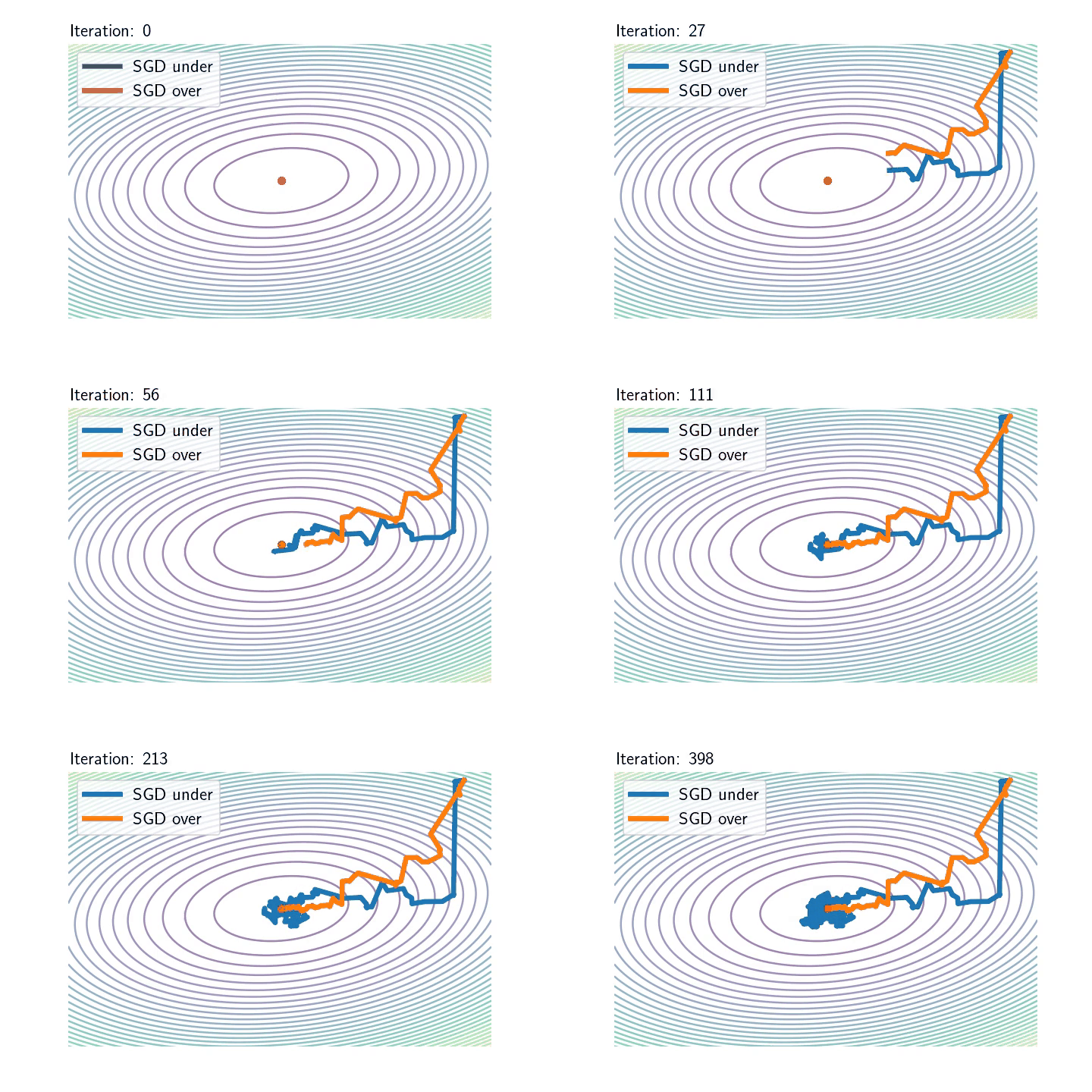
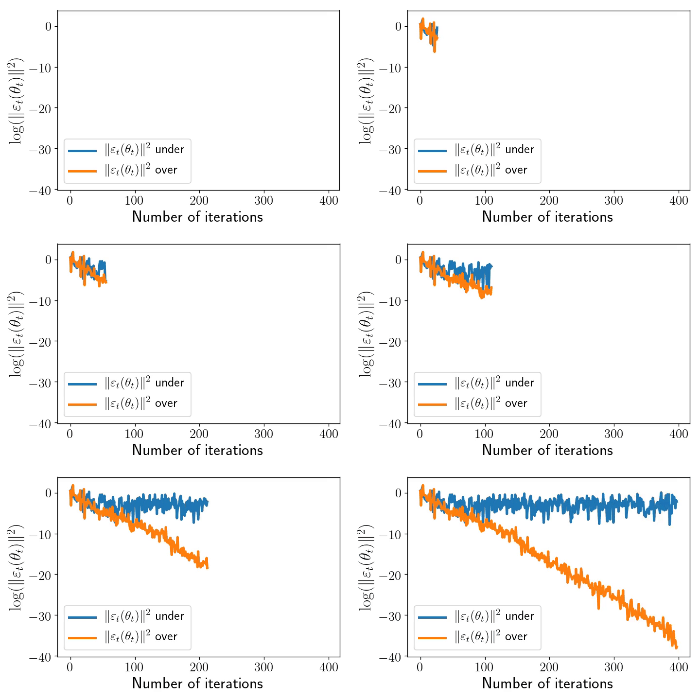
Left: Iterates of SGD for underparametrised (blue) and overparametrised (orange) regimes. The ellipses represent different level sets of \(\mathcal{R}_n\). Inputs \((x_i)_{i\leqslant n}\) are the same in the two models: centred Gaussian with anisotropic covariance (\(n=100,\ d = 2\)). In the underparametrised setting, the outputs have been generated randomly, and there is no interpolator of the dataset, whereas in the overparametrised problem, we generated the outputs according to \(Y = X \theta^* \), where \(\theta^*\) is the unique global minimum of the first setup and hereby of the second as well.
Right: The \(\ell_2\)-norm of the SGD noise in \(\mathrm{log}\)-scale along iterations in the underparametrised (blue) and overparametrised (orange) regimes. In the underparametrised regime, the noise stays constant after \(\sim 75\) iterations, whereas the intensity of the noise goes to \(0\) linearly over the iterates.
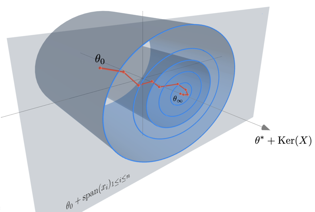
Noise geometry. Another important fact to stress concerning the noise \(\varepsilon_t(\theta)\) is that, at state \(\theta\), it belongs to a specific linear space: \(\text{span}\{\nabla_\theta h(\theta, x_1), …, \nabla_\theta h(\theta, x_n) \}\). To provide an intuition on how restrictive it can be, consider once again our favourite linear model: in this case, \(\nabla_\theta h(\theta, x_i)=x_i\) and \(\varepsilon_t(\theta)\) belongs to \(\text{span}\{x_1, …, x_n \}\), which is a space of dimension at most \(n\). In the overparametrised case, this is a strict subspace of \(\mathbb{R}^d\): noise is degenerate in \(d-n\) directions! On the contrary, in the underparametrised setting, as \(d \leqslant n\) there is no specificity at this level.
SGD as a Markov chain
In this section, we develop a different point of view on the general SGD algorithm, that also provides helpful intuition: we try to understand its dynamics through a Markov chain interpretation.
The first key to understand the behaviour of SGD is that, with constant step-sizes \(\gamma_t = \gamma\), the iterates define an homogeneous Markov chain [4]. Let us recall the SGD recursion to keep it next to us.$$ \theta_t = \theta_{t-1} – \gamma\nabla \mathcal{R}_n (\theta_{t-1}) + \gamma\varepsilon_t(\theta_{t-1}). $$ This point of view induces a natural question: does the distribution of the iterates converge to some limit we can characterise? This will again depend on the regime: under or overparametrised. Roughly, for the former, with a constant step size \(\gamma\), the distribution will converge to a stationary distribution with a strictly positive variance (e.g. a Gaussian centred around \(\theta^*\) at scale \(\gamma^{1/2}\) [5]). Less understood is the fact that, for the latter, it will converge to a Dirac distribution \(\delta_{ \theta^*}\), with \(\theta^*\) being one specific interpolator, that will depend on the precise structure of the algorithm (initialisation, set-size, architecture of the model… more details on this will be discussed in a future blog post)!
The underparametrised case. Recall that in this case, the additive noise is nondegenerate. Hence, the gradient and noise parts of the dynamics cannot cancel simultaneously and under some mild assumption on \(\mathcal{R}_n\), the dynamics equilibrates after a certain time: formally this means that the distribution of the iterates \((\theta_t)_{t \geqslant 0}\) converges to an invariant distribution \(\pi^\gamma\). Hence the question: how far is \(\pi^\gamma\) from \(\delta_{\theta^*}\)? Giving a general and precise answer to this question is not trivial, and more importantly, it depends heavily on the multiplicative part of the noise. For now, let us stick with some common modelling to study the recursion: we make the assumption that the noise does not depend on the current iterate \(\theta\) (multiplicative part is \(0\)). In this case, it has been shown that the iterates of SGD have Gaussian fluctuations around \(\theta^*\) at scale \(\gamma^{1/2}\) [5]. From this point of view, the smaller \(\gamma\), the closer to \(\theta^*\) we get and this justifies a known variance reduction technique: decaying step-sizes. Another technique to reduce the variance is to resort to averaging. Once again, to explain this, ergodic theorems for Markov chains [4] give us an important insight: the time-mean \(\bar{\theta}_t = \frac{1}{t+1} \sum_{i = 0}^t \theta_i\) converges to \(\bar{\theta}_\gamma = \mathbb{E}_{\pi^\gamma} [\theta]\) almost surely. Furthermore, some magic happens with the quadratic case, as we can show that \(\bar{\theta}_\gamma = \theta^*\), which implies, as a direct application of the strong law of large numbers, that \(\bar{\theta}_t\) converges almost surely to \(\theta^*\), and proves that averaging the iterates is relevant [6].
Here is a series of plots corresponding to different step-sizes \(\gamma\) showing the dynamics of plain SGD (blue), averaged SGD (red) and step-sizes decay at \(1/\sqrt{t}\) rate (orange) in an underparametrised setting (\(n=100\), \(d=2\)). Plain SGD is always faster that the other two methods but the larger the \(\gamma\) the larger the variance at optimum is.
Note also that the same analysis can be done in the convex, yet nonquadratic case, indeed, in [7] the authors showed that the order of magnitude of the distance between \(\bar{\theta}_\gamma\) and \({\theta}^*\) is \(\gamma^2\).
The overparametrised case. We have seen in the previous section that both the scale of noise and the geometry are affected in this case. The effect of the geometry is a little bit difficult to handle at a general level and we will detail its role in specific examples (see below and in the next blog post to come). Concerning the scale, we have seen that the noise vanishes at a global optimum and that the closer to a global optimum, the smaller the intensity of the noise is. Hence, global optima are fixed points of the dynamics, and under technical assumptions (e.g. local attractiveness), it can be shown the dynamics eventually converge to one of them [8, 9]. In this case, the nature of the dynamics is very different from the previous one: the distribution of the iterates \((\theta_t)_{t \geqslant 0}\) converges to \(\delta_{\theta^*}\) where \(\theta^*\) is a random variable in the set of interpolators! Remarkably, no variance reduction technique are required for convergence towards a global minimum!
The stochastic gradient flow and the least-squares example
Continuous time model of SGD. Continuous time counterparts of (discrete) numerical optimisation methods and Markov chains are well-worn subjects in applied mathematics and have found applications in machine learning in particular. Indeed, in recent years, gradient descent has been actively studied through gradient flows, which have led to convergence results for neural networks discussed in previous blog posts. However, due to its stochasticity, SGD cannot be properly modelled as a deterministic flow. An interesting and natural approach is to consider stochastic differential equations (SDEs) $$ d \theta_t = b(t,\theta_t) d t + \sigma(t,\theta_t)d B_t, $$ where \((B_t)_{t \geqslant 0}\) is a standard Brownian motion [10]. In order to accurately represent the SGD dynamics, the drift term \(b\) and the noise \(\sigma\) should meet the following requirements:
(i) The drift term \(b\) should match the negative full gradient: \(b=-\nabla \mathcal{R}_n\).
(ii) The noise covariance \(\sigma\sigma^\top(t,\theta)\) should match \(\gamma\mathbb{E}[ \varepsilon_t(\theta_t) \varepsilon_t(\theta_t)^\top | \theta_t = \theta ]\).
(iii) The noise at state \(\theta\) should belong to \(\text{span}\{\nabla_\theta h(\theta, x_1), …, \nabla_\theta h(\theta, x_n) \}\).
\({\color{white} f} \)
Points (i) and (ii) imply that the SGD recursion corresponds in fact to the Euler-Maruyama discretisation with step-size \(\gamma\) of the SDE [11]. Hence, the SDE and the discrete models match perfectly for infinitesimal step-sizes (up to first order terms in \(\gamma\)) and the model is said to be consistent. Point (iii) states a geometrical property of the SGD noise and is of crucial importance for a proper modelisation.
The least-squares model. Consider once again our favourite least-squares model $$\mathcal{R}_n(\theta)= \frac{1}{2n}\sum_{i=1}^n (\langle \theta,x_i\rangle\, – y_i)^2,$$ and let \(X:= [x_1, …, x_n]^\top \in \mathbb{R}^{n \times d}\) be the data matrix and \(y = [y_1, …, y_n]^\top \in \mathbb{R}^n\) the vector of outputs. Let us explicitly write the SDE model in this case: the drift corresponds to the gradient \(b(\theta)=- \frac{1}{n}X^\top (X\theta – y) \) and it is simple linear algebra to calculate the covariance of the noise (see also [19, Remark 4])$$ \sigma \sigma^\top(\theta) = \frac{\gamma}{n} X^\top \left(\textrm{diag}\left[ \big(\langle \theta, x_i\rangle\, – y_i\big)^2 \right]_{i=1}^n – \frac{1}{n} \left[ \big(\langle \theta, x_i\rangle\, – y_i\big)\big(\langle \theta, x_j\rangle\, – y_j\big) \right]_{i,j=1}^n \right) X. $$ To simplify a bit this analysis let us neglect the residual term of order \(1/n^2\) and assume that the residuals \(\langle \theta, x_i\rangle – y_i\), are approximately equal across all the samples of the data set: \(\textrm{diag}\left[ \left(\langle \theta, x_i\rangle\, – y_i\right)^2 \right]_{i=1}^n \simeq \frac{1}{n}\|X \theta\, – y\|^2 I_n \). Then the SDE model writes: $$d \theta_t =\, – \frac{1}{n}X^\top (X\theta_t\, – y) d t + \frac{\sqrt{\gamma}}{n} \| X\theta_t -y \| X^\top d B_t. $$ As stressed before, notice that there is an important difference between the under and overparametrised regimes: in the former, the noise spans all \(\mathbb{R}^d\) and as there exists \(\sigma > 0\) such that \(\| X\theta_t -y \| \geqslant \sigma \), the noise is non degenerate in every direction. Instead, in the overparametrised regime, the noise vanishes at a global optimum \(\theta^*\) and is degenerate in the directions of \([\mathrm{range} (X^\top)]^\perp = \mathrm{Ker} (X)\). As also noticed in [19], this will result in important differences in term of the processes’ behaviour! In the rest of the post, let us denote \(\theta^{\text{LS}}:= X^\dagger y\), where \(X^\dagger\) is the pseudo inverse of \(X\). It corresponds to the ordinary least-square estimator in the underparametrised regime and the projection of \(0\) into \(\mathrm{Ker} (X)\) in the overparametrised setting.
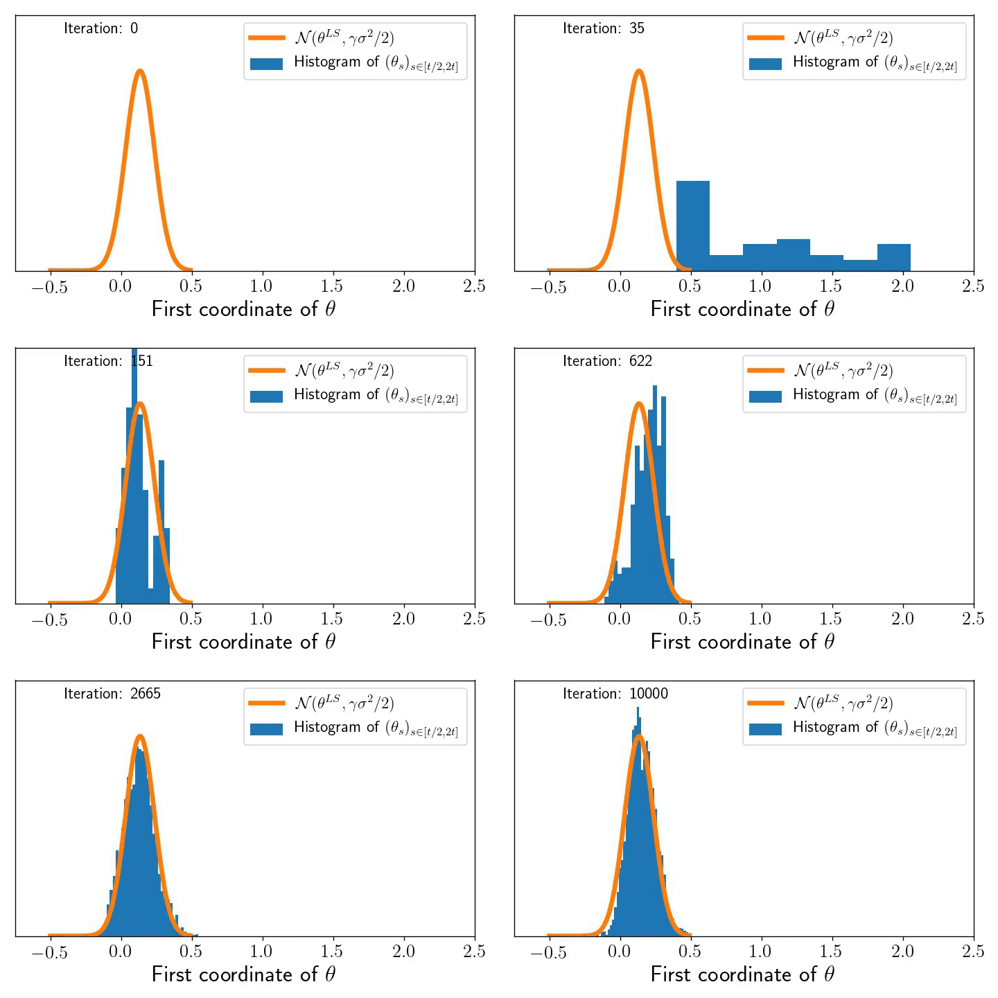
The underparametrised regime and the multivariate Ornstein–Uhlenbeck process. As written before, let us consider a model where the residuals scale like the best possible fit, i.e. \(\frac{1}{\sqrt{n}}\| X\theta_t -y \| \simeq \sigma \). The dynamics reads: $$ d \theta_t =\, – \frac{1}{n}X^\top (X\theta_t\, – y) d t + \sqrt{\frac{\gamma}{n}} \sigma X^\top d B_t. $$ This can be viewed as a multivariate Ornstein–Uhlenbeck process for which we can show the following convergence result: the law \(\pi_t\) of \(\theta_t\) converges to \(\pi^\gamma\), a Gaussian distribution of mean \(\theta^{\text{LS}}\) and covariance \(\frac{\gamma \sigma^2}{2} I_d\): $$\lim_{t \to \infty} \pi_t =\mathcal{N} \left( \theta^{\text{LS}}, \frac{\gamma \sigma^2}{2} I_d \right).$$ From this, as for the Markov chain interpretation, we can nicely interpret the need to decrease step-sizes to \(0\) in order to concentrate to \(\theta^{\text{LS}}\). Similarly, note that the ergodic theorem gives you automatically that the time average of \(\theta_t\) goes to \(\theta^{\text{LS}}\) as $$\qquad \qquad \qquad \lim_{t \to \infty} \frac{1}{t}\int_0^t \theta_s ds = \mathbb{E}[\pi^\gamma]=\theta^{\text{LS}}, \qquad \text{almost surely}.$$ Besides its nice interpretation as a Ornstein-Uhlenbeck process, we illustrate below the predictive power of the SDE model to understand the SGD dynamics.

Left: \(10\) realisations of SGD in blue-like colours (corresponding to \(10\) different random sampling sequences), next to \(10\) realisations of the SDE model in red-like colours (corresponding to \(10\) different realisations of the Brownian motion).
Right: A histogram of snap-shots of the SGD dynamics (marginal along the first coordinate) at increasing time intervals that show the convergence (by ergodicity) to the predicted Gaussian \(\mathcal{N}(\theta^{\text{LS}}, \gamma \sigma^2/2)\) !
The overparametrised regime and the geometric Brownian motion. We take back our SDE model, initialise it at \(\theta_0 = 0\), but now we are extra careful that the noise cancels at any interpolator \(\theta^*\). We will show that despite being a random process, the dynamics with constant \(\gamma > 0\) converges almost surely to \(\theta^{\text{LS}}\). To do so let us consider the evolution of the squared difference \(\eta_t = \|\theta_t – \theta^{\text{LS}}\|^2\). Thanks to Itô calculus (chain rule for stochastic processes), $$\begin{aligned} d \eta_t &= 2 \langle d \theta_t, \theta_t – \theta^{\text{LS}} \rangle + \frac{\gamma}{n^2} \mathrm{tr} (X^\top X) \| X (\theta_t – \theta^{\text{LS}}) \|^2 dt \\ &= 2\left( \gamma \mathrm{tr} \left(n^{-1}X^\top X\right) – 2 \right) \mathcal{R}_n(\theta_t) dt + 4\sqrt{\gamma}\mathcal{R}_n(\theta_t) dW_t, \end{aligned} $$ where \((W_t)_{t \geqslant 0}\) is a one dimensional Brownian motion (see details of this calculation at the end of the post). To simplify the calculation set the step-size such that \(\gamma \mathrm{tr} (n^{-1}X^\top X) = 1\) (note that we retrieve here the usual step-size for least-squares SGD [16]). Noting \(\mu_t = \frac{2\mathcal{R}_n(\theta_t)}{\eta_t}\) and \(\nu_t = \frac{4\sqrt{\gamma}\mathcal{R}_n(\theta_t)}{\eta_t}\), the dynamics of \((\eta_t)_{t \geqslant 0}\) follows $$d \eta_t = -\mu_t \eta_t dt + \nu_t \eta_t dW_t, $$ Furthermore, as \(\theta_t – \theta^{\text{LS}} \in \mathrm{span} (X^\top)\) , we have \(\mu\cdot \eta_t\leqslant 2 \mathcal{R}_n(\theta_t) \leqslant L\cdot \eta_t\), where \(\mu\) and \(L\) stand respectively for the minimum and maximum eigenvalues of \(\frac{1}{n}XX^\top\). Hence, the behaviour of \((\eta_t)_{t \geqslant 0}\) is approximately the same as that of the solution to the following SDE: $$d S_t = -\mu S_t dt + \nu S_t dW_t, $$ for \(\nu \simeq 4 L \sqrt{\gamma}\). That is, the dynamics of \((\|\theta_t – \theta^{\text{LS}}\|^2)_{t \geqslant 0}\) is approximately the one of a Geometric Brownian Motion (GBO), a.k.a. the process underlying the Black-Scholes model! Hence, to understand SGD in the overparametrised regime, one “simply” need to study the properties of the GBO. It is known that in fact there is an explicit solution of this SDE $$ S_t = S_0 \exp\left( -\left(\mu + \frac{\nu^2}{2}\right) t + \nu W_t\right). $$ Hence, for all \(t>0\), \(S_t\) is distributed according to a log-normal random variable with mean \(\mathbb{E}(S_t) = S_0 e^{- \mu t}\) and variance \(\text{var}(S_t) = S_0^2 e^{- 2\mu t} (e^{\nu^2 t} – 1)\). Furthermore, it is a nice application to the law of the iterated logarithm for the Brownian motion to show that $$ \qquad \qquad \qquad \lim_{t \to \infty} S_t = 0, \qquad \text{almost surely!} $$ The almost sure convergence of \((\theta_t)_{t \geqslant 0}\) to \(\theta^{\text{LS}}\) is in stark contrast with the limiting behaviour we have seen in the underparametrised setting. Remarkably, the process does not require any variance reduction to converge to a specific point. Note also that among all the possible interpolators the process could have converged to, the process in fact goes almost surely to \(\theta^{\text{LS}}\). This selection of the minimum norm interpolator [12], known as the implicit bias of the process will be the core of a next blog post (for more complex architectures).
As in the underparametrised case, below are two plots showing the typical behaviour of the SGD dynamics as a GBO.
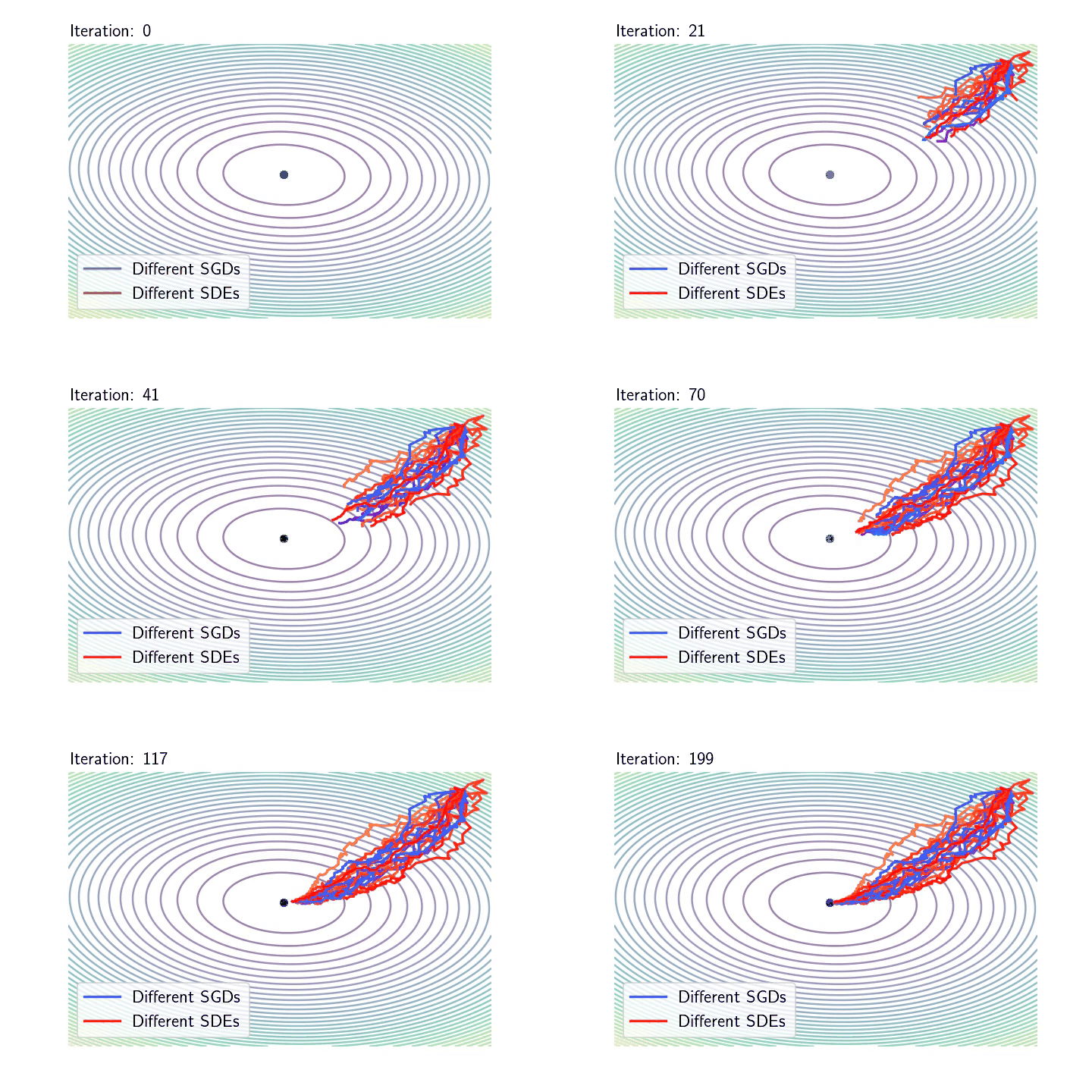
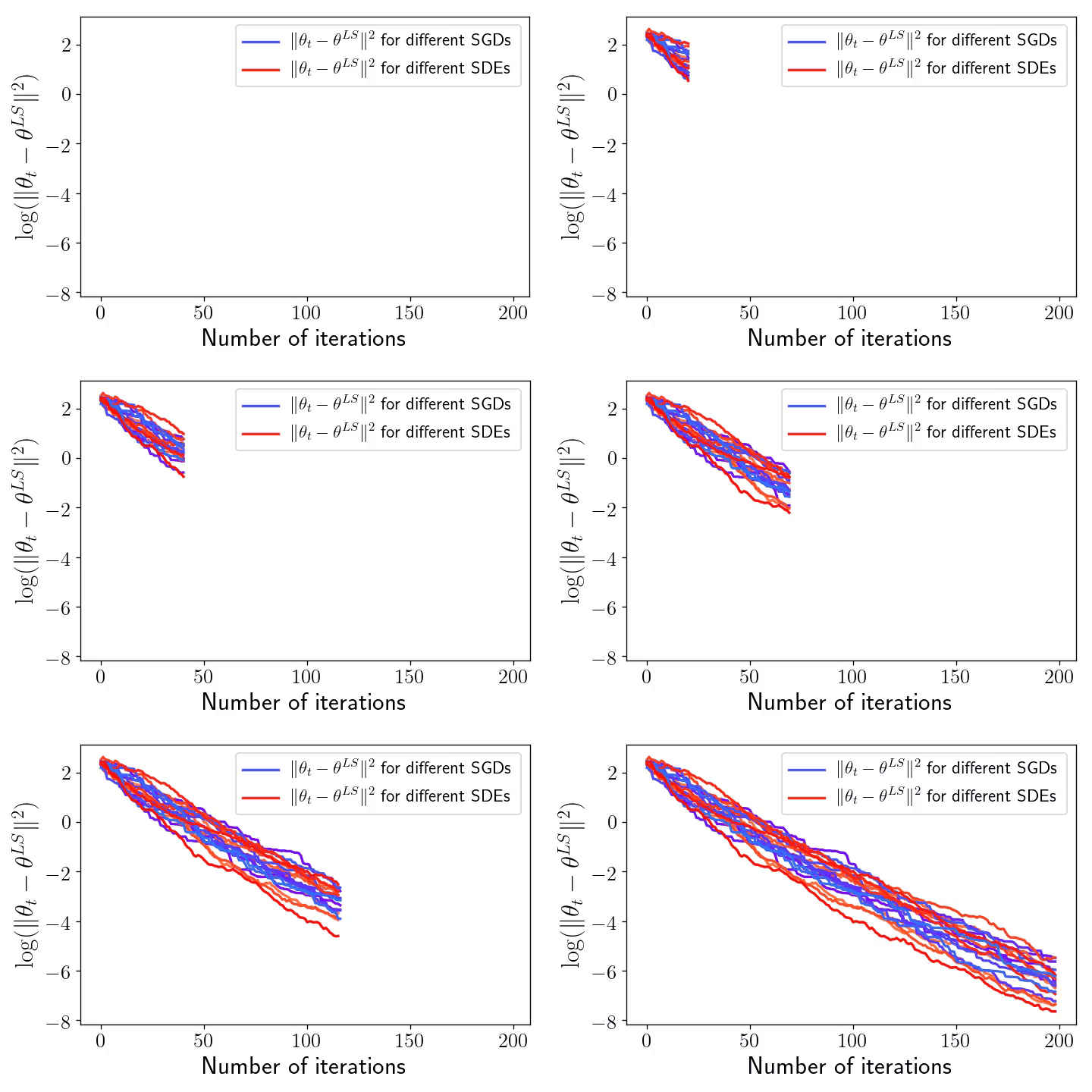
Left: \(10\) realisations of SGD in blue-like colours (corresponding to \(10\) different random sampling sequences), next to \(10\) realisations of the SDE model in red-like colours (corresponding to \(10\) different realisations of the Brownian motion).
Right: The exponential convergence of \(\eta_t = \|\theta_t – \theta^{\text{LS}}\|^2\) to \(0\) for the \(10\) realisations of SGD and the SDE (in log-scale).
Conclusion
In this blog post, I have tried to show that despite the old legacy inherited from the stochastic approximation literature, the particularities of the noise of the stochastic gradient descent in machine learning contexts necessitate a fresh look. This specificity strikes the most in modern overparametrised models as the noise can be largely degenerate, both (i) in direction (which I called noise geometry), and (ii) in scale, as its variance is dominated by the loss and hence vanishes at a global optimum. In fact I have tried to show that SDE models can be a relevant framework to shed light on typical behaviours of stochastic learning dynamics: for overparametrised architectures, they differentiate from the overdamped Langevin diffusion model, and act as multiplicative noise dynamics like the geometric brownian motion.
Besides, as it is believed that stochasticity plays a role in the generalisation performances of optimisation algorithms [13], there is a need to consider its action precisely. Yet, grasping its overall nature appears to be particularly hard as it mixes properties from the model’s architecture, the data’s distribution and the loss. In a following post, I will try to analyse some simple non-convex models where we can show that the SGD-noise drives the dynamics to possibly “good for generalisation” regions [17,18].
Acknowledgements. I would like to thank Scott Pesme and Etienne Boursier for fruitful discussions, and especially Nicolas Le Hir for proofreading this blog post and making good clarifying suggestions.
References
[1] Herbert Robbins and Sutton Monro. A Stochastic Approximation Method. The Annals of Mathematical Statistics, 22 (3): 400 – 407, September, 1951.
[2] Marie Duflo. Algorithmes stochastiques. Volume 23 of Mathématiques & Applications (Berlin) [Mathematics & Applications]. Springer-Verlag, Berlin, 1996
[3] Léon Bottou and Olivier Bousquet. The Tradeoffs of Large Scale Learning, In Advances in Neural Information Processing Systems, vol.20, 161-168, 2008.
[4] Sean P.Meyn and Richard L. Tweedie. Markov Chains and Stochastic Stability. Springer, London, 1993.
[5] Georg Ch. Pflug. Stochastic minimization with constant step-size: asymptotic laws. SIAM Journal on Control and Optimization, 24(4):655–666, 1986.
[6] Francis Bach and Eric Moulines. Non-asymptotic analysis of stochastic approximation algorithms for machine learning. In Advances in Neural Information Processing Systems (NIPS), 2011.
[7] Aymeric Dieuleveut, Alain Durmus and Francis Bach. Bridging the gap between constant step size stochastic gradient descent and Markov chains. The Annals of Statistics, 48 (3): 1348 – 1382, June 2020.
[8] Stephan Wojtowytsch. Stochastic gradient descent with noise of machine learning type. Part I: Discrete time analysis Technical Report, arXiv-2105.01650, 2021.
[9] Aditya Varre, Loucas Pillaud-Vivien and Nicolas Flammarion. Last iterate convergence of SGD for Least-Squares in the Interpolation regime. Advances in Neural Information Processing Systems 34, 21581-21591, 2021.
[10] Bernt Øksendal. Stochastic Differential Equations: An Introduction with Applications, 6th edition. Springer, New York, 2003.
[11] Qianxiao Li, Cheng Tai, and Weinan E. Stochastic modified equations and dynamics of stochastic gradient algorithms i: Mathematical foundations. Journal of Machine Learning Research, 20(40):1–47, 2019.
[12] Chiyuan Zhang, Samy Bengio, Moritz Hardt, Benjamin Recht, and Oriol Vinyals. Understanding deep learning requires rethinking generalization. In International Conference on Learning Representations, 2017.
[13] Nitish Shirish Keskar, Dheevatsa Mudigere, Jorge Nocedal, Mikhail Smelyanskiy, and Ping Tak Peter Tang. On large-batch training for deep learning: Generalization gap and sharp minima. In International Conference on Learning Representations, 2017.
[14] Sharan Vaswani, Francis Bach and Mark Schmidt. Fast and Faster Convergence of SGD for Over-Parameterized Models and an Accelerated Perceptron. Proceedings of the Twenty-Second International Conference on Artificial Intelligence and Statistics, PMLR 89:1195-1204, 2019.
[15] Siyuan Ma, Raef Bassily and Mikhail Belkin. The Power of Interpolation: Understanding the Effectiveness of SGD in Modern Over-parametrized Learning. Proceedings of the 35th International Conference on Machine Learning, PMLR 80:3325-3334, 2018.
[16] Alexandre Defossez and Francis Bach. Averaged Least-Mean-Squares: Bias-Variance Trade-offs and Optimal Sampling Distributions. Proceedings of the Eighteenth International Conference on Artificial Intelligence and Statistics, PMLR 38:205-213, 2015.
[17] Scott Pesme, Loucas Pillaud-Vivien and Nicolas Flammarion. Implicit bias of SGD for diagonal linear networks: a provable benefit of stochasticity. In Advances in Neural Information Processing Systems 34, 29218-29230, 2021.
[18] Loucas Pillaud Vivien, Julien Reygner and Nicolas Flammarion. Label noise (stochastic) gradient descent implicitly solves the Lasso for quadratic parametrisation. Proceedings of Thirty Fifth Conference on Learning Theory, PMLR 178:2127-2159, 2022.
[19] Alnur Ali, Edgar Dobriban and Ryan Tibshirani. The Implicit Regularization of Stochastic Gradient Flow for Least Squares. Proceedings of the 37th International Conference on Machine Learning, PMLR 119:233-244, 2020.
Details on the evolution equation of \(\eta_t = \|\theta_t – \theta^{\text{LS}}\|^2\).
Recall that the evolution of the iterates is given by the SDE: $$ d \theta_t =\, – \frac{1}{n}X^\top (X\theta_t\, – y) d t + \frac{\sqrt{\gamma}}{n} \| X\theta_t -y \| X^\top d B_t. $$ Then by Itô calculus, we have $$\begin{aligned} d \eta_t &= 2 \langle d \theta_t, \theta_t – \theta^{\text{LS}} \rangle + \frac{\gamma}{n^2} \mathrm{tr} (X^\top X) \| X (\theta_t – \theta^{\text{LS}}) \|^2 dt \\ &= -\frac{2}{n} \langle X^\top (X\theta_t\, – y), \theta_t – \theta^{\text{LS}} \rangle dt + 2 \sqrt{\frac{2\gamma}{n}} \sqrt{\mathcal{R}_n(\theta_t)} \langle X^\top d B_t, \theta_t – \theta^{\text{LS}} \rangle \\ & \hspace{6.5cm}+ 2\gamma \mathrm{tr} (n^{-1}X^\top X) \mathcal{R}_n(\theta_t) dt. \end{aligned}$$ Since, \(\theta^{\text{LS}}\) is an interpolator, i.e \(X \theta^{\text{LS}} = y\), the first term corresponds to $$ -\frac{2}{n}\langle X^\top (X\theta_t\, – y), \theta_t – \theta^{\text{LS}} \rangle = -\frac{2}{n}\langle X(\theta_t – \theta^{\text{LS}}), X(\theta_t – \theta^{\text{LS}}) \rangle = -4 \mathcal{R}_n(\theta_t).$$ For the second term, note that \(\langle X^\top d B_t, \theta_t – \theta^{\text{LS}} \rangle = \langle d B_t, X(\theta_t – \theta^{\text{LS}}) \rangle\), and by Lévy’s Characterization of Brownian Motion, the local martingale $$ W_t = \int_0^t \frac{\langle d B_s, X(\theta_s – \theta^{\text{LS}})\rangle}{\|X(\theta_s – \theta^{\text{LS}})\|} $$ is in fact a one dimensional Brownian motion. Hence, $$ \langle X^\top d B_t, \theta_t – \theta^{\text{LS}} \rangle = \|X(\theta_s – \theta^{\text{LS}})\| dW_t = \sqrt{2 n \mathcal{R}_n(\theta_t)}dW_t,$$ and finally, $$ d \eta_t = -4 \mathcal{R}_n(\theta_t) dt + 4 \sqrt{\gamma} \mathcal{R}_n(\theta_t) d W_t + 2 \gamma \mathrm{tr} (n^{-1}X^\top X) \mathcal{R}_n(\theta_t) dt,$$ which gives the claimed result of the main text.
Hi Loucas, I wrote a short paper https://arxiv.org/abs/2007.09286
a couple years ago where I analyzed the training dynamics for deep linear networks using a new metric – layer imbalance – which defines the flatness of a solution. I demonstrated that different regularization methods, such as weight decay or noise data augmentation, behave in a similar way. Training has two distinct phases: 1) optimization and 2) regularization. First, during the optimization phase, the loss function monotonically decreases, and the trajectory goes toward a minima manifold. Then, during the regularization phase, the layer imbalance decreases, and the trajectory goes along the minima manifold toward a flat area. I also showed that SGD works similarly to noise regularization.
Hi, thanks a lot for this post!
I’m just a bit confused by the caption on your first figure: you say “In the underparametrised setting, the outputs have been generated randomly”, which is a bit confusing since the blue trajectory still goes towards the solution, plus that doesn’t really match the point you make in the text? I would have expected as illustration the model where e.g theta_1 is fixed (and != theta*_1) and only theta_2 is trained…
(Also in §References, [13] and [8] are on the same line somehow)
Hi Guillaume, thanks for the comment and the typo.
You are totally right that I could have detailed a bit more the setup. Let me try to make it clearer:
– In the underparametrised case, the output vector Y is a standard gaussian and the training loss R_n has a positive global minimum that is attained uniquely in \theta^*=\theta^{LS}, the ordinary least-squares estimator defined in the last section. As shown later, it is expected that the blue trajectory indeed goes to the solution \theta^{LS} but suffers from some positive variance when approaching it. This is the reason why it seems to bounce around it.
– In the overparametrised case, the inputs are the same but I generated the output according to \theta^*=\theta^{LS}, i.e. \tilde{Y} = X\theta^{LS}. Hence, even if the minimiser of the train loss is the same as in the underparametrised setup, a crucial change occurs: the global minimum is zero in this case! Hence the important point is that there is no positive variance when approaching the solution. Finally, I admit that what might be confusing is the “overparametrised” word: in fact this is the existence of a perfect interpolator that changes the overall behaviour (that often coincide with the overparametrised regime… but not in this precise case).
Greetings! Very helpful advice within this article! It is the little changes that will make the most significant changes. Thanks a lot for sharing!