On the unreasonable effectiveness of Richardson extrapolation

This month, I will follow up on last month’s blog post, and describe classical techniques from numerical analysis that aim at accelerating the convergence of a vector sequence to its limit, by only combining elements of the sequence, and without the detailed knowledge of the iterative process that has led to this sequence.

Last month, I focused on sequences that converge to their limit exponentially fast (which is referred to as linear convergence), and I described Aitken’s \(\Delta^2\) method, the Shanks transformation, Anderson acceleration and its regularized version. These methods are called “non-linear” acceleration techniques, because, although they combine linearly iterates as \(c_0 x_k + c_1 x_{k+1} + \cdots + c_m x_{k+m}\), the scalar weights in the linear combination depend non-linearly on \(x_k,\dots,x_{k+m}\).

In this post, I will focus on sequences that converge sublinearly, that is, with a difference to their limit that goes to zero as an inverse power of \(k\), typically in \(O(1/k)\).

Richardson extrapolation

We consider a sequence \((x_k)_{k \geq 0} \in \mathbb{R}^d\), with an asymptotic expansion of the form $$ x_k = x_\ast + \frac{1}{k}\Delta + O\Big(\frac{1}{k^2}\Big), $$ where \(x_\ast \in \mathbb{R}^d\) is the limit of \((x_k)_k\) and \(\Delta\) a vector in \(\mathbb{R}^d\).

The idea behind Richardson extrapolation [1] is to combine linearly two iterates taken at two different values of \(k\) so that the zero-th order term \(x_\ast\) is left unchanged, but the first order term in \(1/k\) cancels out. For \(k\) even, we can consider $$ 2 x_k – x_{k/2} = 2 \Big( x_\ast + \frac{1}{k} \Delta  +O\Big(\frac{1}{k^2}\Big)  \Big) \, – \Big( x_\ast +  \frac{2}{k} \Delta  + O\Big(\frac{1}{k^2}\Big) \Big) = x_\ast +O\Big(\frac{1}{k^2}\Big).$$

The key benefit of Richardson extrapolation is that we only need to know that the leading term in the asymptotic expansion is proportional to \(1/k\), without the need to know the vector \(\Delta\). See an illustration below.

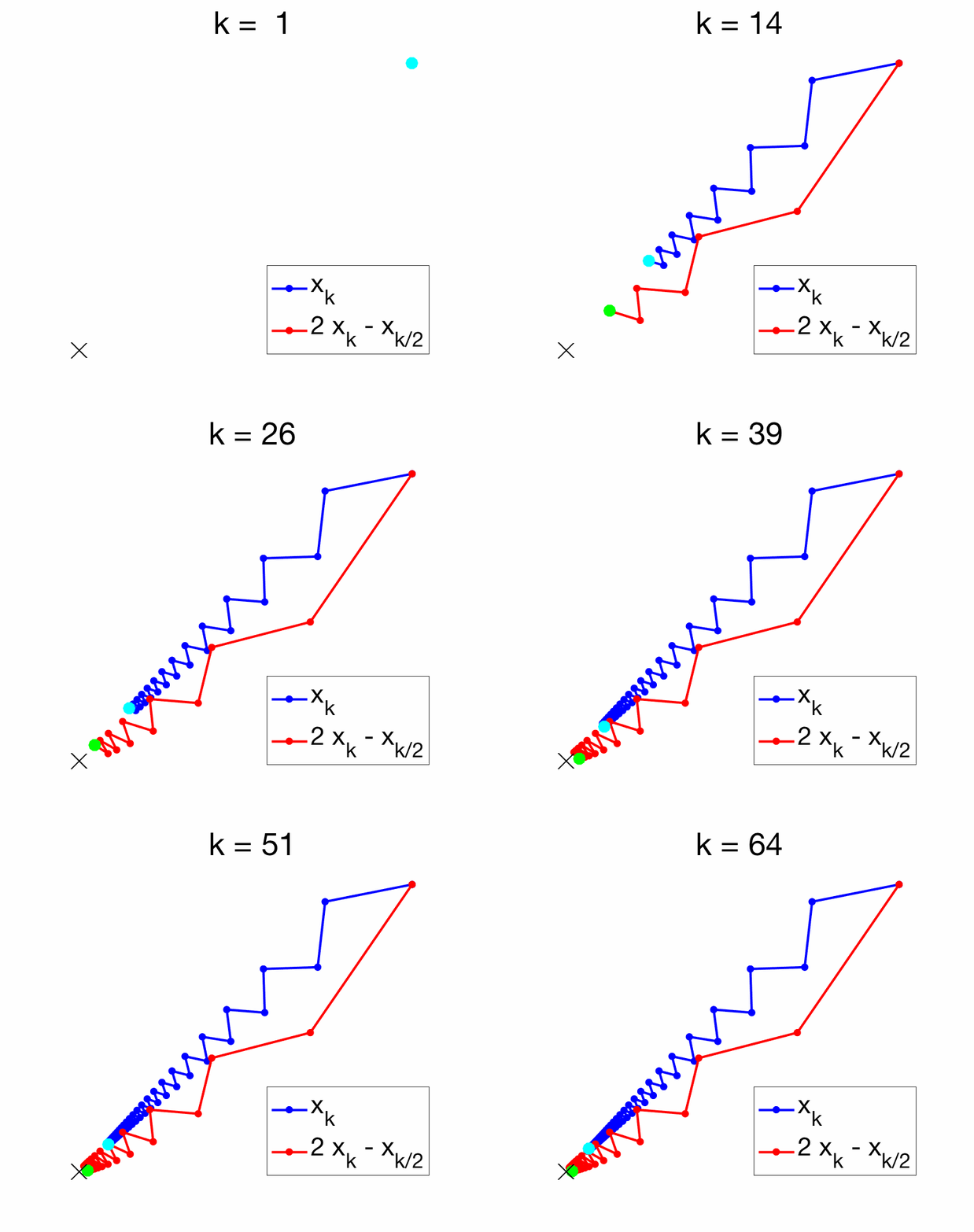
In this post, following [2], I will explore situations where Richardson extrapolation can be useful within machine learning. I identified three situations where Richardson extrapolation can be useful (there are probably more):

1. Iterates of an optimization algorithms \((x_k)_{k \geq 0}\), and the extrapolation is \( 2x_k – x_{k/2}.\)
2. Extrapolation on the step-size of stochastic gradient descent, where we will combine iterates obtained from two different values of the step-size.
3. Extrapolation on a regularization parameter.

As we will show, extrapolation techniques come with no significant loss in performance, but in several situations strong gains. It is thus “unreasonably effective“.

Application to optimization algorithms

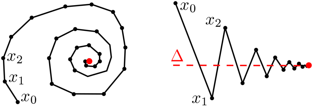
We consider an iterate \(x_k\) of an iterative optimization algorithm which is minimizing a function \(f\), thus converging to a global minimizer \(x_\ast\) of \(f\). Then so is \(x_{k/2}\), and thus also $$ x_k^{(1)} = 2x_k – x_{k/2}.$$ Therefore, performance is never significantly deteriorated (the risk is essentially to lose half of the iterations). The potential gains depend on the way \(x_k\) converges to \(x_\ast\). The existence of a convergence rate of the form \(f(x_k) -f(x_\ast) = O(1/k)\) or \(O(1/k^2)\) is not enough, as Richardson extrapolation requires a specific direction of asymptotic convergence. As illustrated below, some algorithms are oscillating around their solutions, while some converge with a specific direction. Only the latter ones can be accelerated with Richardson extrapolation, while the former ones are good candidates for Anderson acceleration.

Averaged gradient descent. We consider the usual gradient descent algorithm $$x_k = x_{k-1} – \gamma f'(x_{k-1}),$$ where \(\gamma > 0 \) is a step-size, with Polyak-Ruppert averaging [4]: $$ y_k = \frac{1}{k} \sum_{i=0}^{k-1} x_i.$$ Averaging is key to robustness to potential noise in the gradients [4, 5]. However it comes with the unintended consequence of losing the exponential forgetting of initial conditions for strongly-convex problems [6].

A common way to restore exponential convergence (up to the noise level in the stochastic case) is to consider “tail-averaging”, that is, to replace \(y_k\) by the average of only the latest \(k/2\) iterates [7]. As shown below for \(k\) even, this corresponds exactly to Richardson extrapolation on the sequence \((y_k)_k\): $$ \frac{2}{k} \sum_{i=k/2}^{k-1} x_i = \frac{2}{k} \sum_{i=0}^{k-1} x_i – \frac{2}{k} \sum_{i=0}^{k/2-1} x_i = 2 y_k – y_{k/2}. $$

With basic  assumptions on \(f\), it is shown in [2] that for locally strongly-convex problems: $$y_k = x_\ast + \frac{1}{k} \Delta + O(\rho^k), $$ where  \(\displaystyle \Delta = \sum_{i=0}^\infty (x_i – x_\ast)\) and \(\rho \in (0,1)\) depends on the condition number of \(f”(x_\ast)\). This is illustrated below.

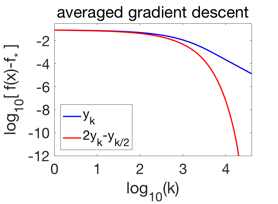
We can make the following observations:

• Before Richardson extrapolation, the asymptotic convergence rate after averaging is of order \(O(1/k^2)\), which is better than the usual \(O(1/k)\) upper-bound for the rate of gradient descent, but with a stronger assumption that in fact leads to exponential convergence before averaging.
• While \(\Delta\) has a simple expression, it cannot be computed in practice (but Richardson extrapolation does not need to know it).
• Richardson extrapolation leads to an exponentially convergent algorithm from an algorithm converging asymptotically in \(O(1/k^2)\).

Accelerated gradient descent. Above, we considered averaged gradient descent, which is asymptotically converging as \(O(1/k^2)\), and on which Richardson extrapolation could be used with strong gains. Is it possible also for the accelerated gradient descent method [8], which has a (non-asymptotic) convergence rate of \(O(1/k^2)\) for convex functions?

It turns out that the behavior of the iterates of accelerated gradient descent is exactly of the form depicted in the left plot of the figure above: that is, the iterates \(x_k\) oscillate around the optimum [9, 10], and Richardson extrapolation is of no help, but is not degrading performance too much. See below for an illustration. 

Other algorithms. It is tempting to test it on other optimization algorithms. For example, as explained in [2], Richardson extrapolation can be used to the Frank-Wolfe algorithm, where sometimes it helps, sometimes it doesn’t. Others could be tried.

Extrapolation on the step-size of stochastic gradient descent

While above we have focused on Richardson extrapolation applied to the number of iterations of an iterative algorithm, it is most often used in integration methods (for computing integrals or solving ordinary differential equations), and then often referred to as Romberg-Richardson extrapolation. Within machine learning, in a similar spirit, this can be applied to the step-size of stochastic gradient descent [3, 11], which I now describe.

We consider the minimization of a function \(F(x)\) defined on \(\mathbb{R}^d\), which can be written as an expectation as $$F(x) = \mathbb{E}_{z} f(x,z).$$ We assume that we have access to \(n\) independent and identically distributed observations (i.i.d.) \(z_1,\dots,z_n\). This is a typical scenario in machine learning, where \(f(x,z)\) represents the loss for the predictor parameterized by \(x\) on the observation \(z\).

The stochastic gradient method is particularly well adapted, and we consider here a single pass, as $$x_i= x_{i-1} – \gamma f'(x_{i-1},z_i),$$ where the gradient is taken with respect to the first variable, for \(i = 1,\dots,n\). It is known that with a constant step-size, when \(n\) tends to infinity, \(x_n\) will not converge to the minimizer \(x_\ast\) of \(F\), as the algorithm always moves [16], as illustrated below.

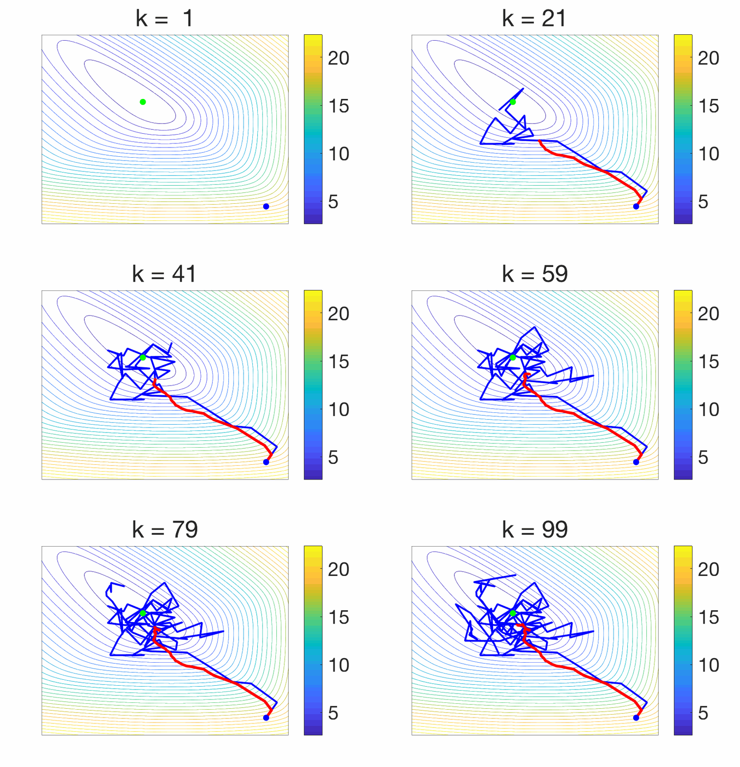
One way to damp the oscillations is to consider averaging, that is, $$ y_n = \frac{1}{n+1} \sum_{i=0}^{n} x_i$$ (we consider uniform averaging for simplicity). For least-squares regression, this leads to a converging algorithm [12] with attractive properties for ill-conditioned problems (see also January’s blog post). However, for general loss functions, it is shown in [3] that \(y_n\) converges to some \(y^{(\gamma)} \neq x_\ast\). There is a bias due to a step-size \(\gamma\) that does not go to zero. In order to apply Richardson extrapolation, together with Aymeric Dieuleveut and Alain Durmus [3], we showed that $$ y^{(\gamma)} = x_\ast + \gamma \Delta + O(\gamma^2),$$ for some \(\Delta \in \mathbb{R}^d\) with some complex expression. Thus, we have $$2 y^{(\gamma)} – y^{(2\gamma)} = x_\ast + O(\gamma^2),$$ thus gaining one order. If we consider the iterate \(y_n^{(\gamma)}\) and \(y_n^{(2 \gamma)}\) associated to the two step-sizes \(\gamma\) and \(2 \gamma\), the linear combination $$2 y_n^{(\gamma)} – y_n^{(2\gamma)} $$ has an improved behavior as it tends to \(2 y^{(\gamma)} – y^{(2\gamma)} = x_\ast + O(\gamma^2)\): it remains not convergent, but get to way smaller values. See an illustration below.

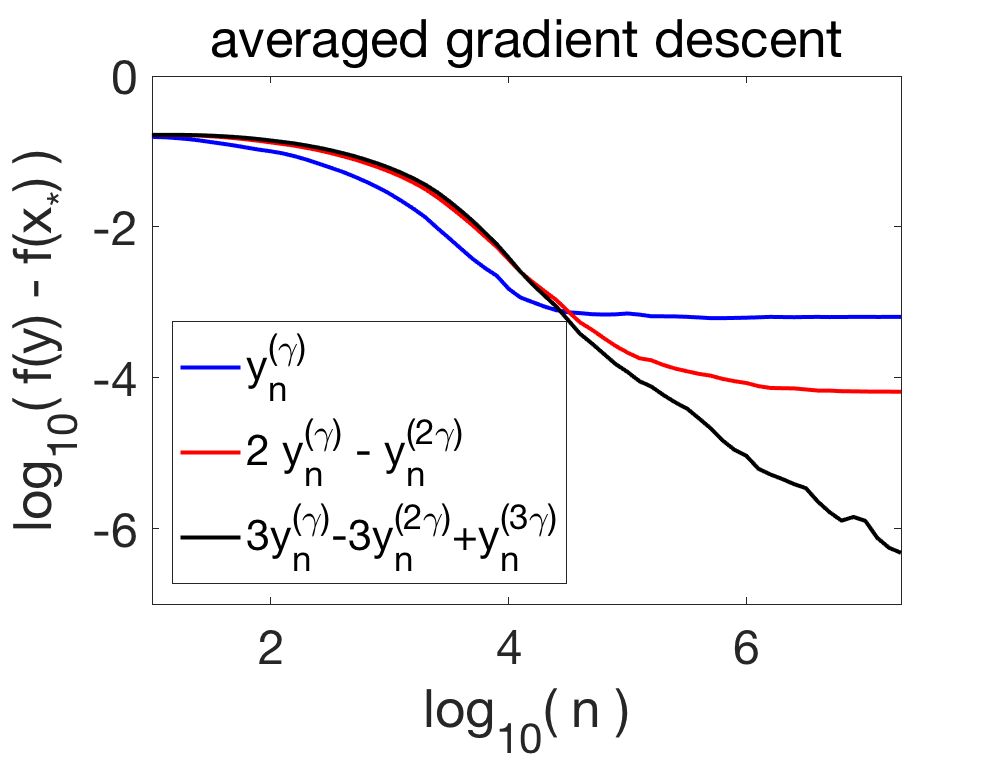
Higher-order extrapolation. If we can accelerate a sequence by extrapolation, why not extrapolate the extrapolated sequence? This is possible if we have an higher-order expansion of the form $$ y^{(\gamma)} = \theta_\ast + \gamma \Delta_1 + \gamma^2 \Delta_2 + O(\gamma^3),$$ for some (typically unknown) vectors \(\Delta_1\) and \(\Delta_2\). Then, the sharp reader can check that $$3 y_n^{(\gamma)} – 3 y_n^{(2\gamma)} + y_n^{(3\gamma)}, $$ will lead to cancellation of the first two orders \(\gamma\) and \(\gamma^2\). This is illustrated above for SGD.

Then, why not extrapolate the extrapolation of the extrapolated sequence? One can check that $$4 y_n^{(\gamma)} – 6 y_n^{(2\gamma)} + 4 y_n^{(3\gamma)} -y_n^{(4\gamma)}, $$ will lead to cancellation of the first three orders of an expansion of \(y^{(\gamma)}\). The binomial coefficient aficionados have already noticed the pattern there, and checked that $$ \sum_{i=1}^{m+1} (-1)^{i-1} { m+1 \choose i} y_n^{(i\gamma)}$$ will lead to cancellations of the first \(m\) orders.

Then, why not go on forever? First because \(m+1\) recursions have to be run in parallel, and second, because the constant in front of the term in \(\gamma^{m+1}\) typically explodes, a phenomenon common to many expansion methods.

Extrapolation on a regularization parameter

We now explore the application of Richardson extrapolation to regularization methods. In a nutshell, regularization allows to make an estimation problem more stable (less subject to variations for statistical problems) or the algorithm faster (for optimization problems). However, regularization adds a bias that needs to be removed. In this section, we apply Richardson extrapolation to the regularization parameter to reduce this bias. I will only present an application to smoothing for non-smooth optimization (see an application to ridge regression in [2]).

Non-smooth optimization problems. We consider the minimization of a convex function of the form \(f = h + g\), where \(h\) is smooth and \(g\) is non-smooth. These optimization problems are ubiquitous in machine learning and signal processing, where the lack of smoothness can come from (a) non-smooth losses such as max-margin losses used in support vector machines and more generally structured output classification [13], and (b) sparsity-inducing regularizers (see, e.g., [14] and references therein). While many algorithms can be used to deal with this non-smoothness, we consider a classical smoothing technique below.

Nesterov smoothing. In this section, we consider the smoothing approach of Nesterov [15] where the non-smooth term is “smoothed” into \(g_\lambda\), where \(\lambda\) is a regularization parameter, and accelerated gradient descent is used to minimize \(h+g_\lambda\). 

A typical way of smoothing the function \(g\) is to add \(\lambda\) times a strongly convex regularizer (such as the squared Euclidean norm) to the Fenchel conjugate of \(g\); this leads to a function \(g_\lambda\) which has a smoothness constant (defined as the maximum of the largest eigenvalues of all Hessians) proportional to \(1/\lambda\), with a uniform error of \(O(\lambda)\) between \(g\) and \(g_\lambda\). Given that accelerated gradient descent leads to an iterate with excess function values proportional to \(1/(\lambda k^2)\) after \(k\) iterations, with the choice of \(\lambda \propto 1/k\), this leads to an excess in function values proportional to \(1/k\), which improves on the subgradient method which converges in \(O(1/\sqrt{k})\). Note that the amount of regularization depends on the number of iterations, so that this smoothing method is not “anytime”.

Richardson extrapolation. If we denote by \(x_\lambda\) the minimizer of \(h+g_\lambda\) and \( x_\ast\) the global minimizer of \( f=h+g\), if we can show that \( x_\lambda = x_\ast + \lambda \Delta + O(\lambda^2)\), then \( x^{(1)}_\lambda = 2 x_\lambda – x_{2\lambda} = O(\lambda^2)\) and we can expand \( f(x_\lambda^{(1)})  = f(x_\ast)  + O(\lambda^2)\), which is better than the \(O(\lambda)\) approximation without extrapolation. 

Then, given a number of iterations \(k\), with \( \lambda \propto k^{-2/3}\), to balance the two terms \( 1/(\lambda k^2)\) and \( \lambda^2\),  we get an overall convergence rate for the non-smooth problem of \( k^{-4/3}\).

\(m\)-step Richardson extrapolation. Like above for the step-size, we can also consider \(m\)-step Richardson extrapolation \(x_{\lambda}^{(m)}\), which leads to a bias proportional to \(\lambda^{m+1}\). Thus, if we consider \(\lambda \propto 1/k^{2/(m+2)}\), to balance the terms \(1/(\lambda k^2)\) and \(\lambda^{m+1}\), we get an error for the non-smooth problem of \(1/k^{2(m+1)/(m+2)}\), which can get arbitrarily close to \(1/k^2\) when \(m\) gets large. The downsides (like for the extrapolation on the step-size above) are that (a) the constants in front of the asymptotic equivalent may blow up (a classical problem in high-order expansions), and (b) \(m\)-step extrapolation requires running the algorithm \(m\) times (this can be down in parallel). In the experiment below, 3-step extrapolation already brings in most of the benefits.

In order to experimentally study the benefits of extrapolation, for the Lasso optimization problem, and for a series of regularization parameters equal to \(2^{i}\) for \(i\) between \(-18\) and \(1\) (sampled every \(1/5\)), we run accelerated gradient descent on \(h+g_\lambda\) and we plot the value of \(f(x)-f(x_\ast)\) for the various estimates, where for each number of iterations, we minimize over the regularization parameter. This is an oracle version of varying \(\lambda\) as a function of the number of iterations.

Conclusion

These last two blog posts were dedicated to acceleration techniques coming from numerical analysis. They are cheap to implement, typically do not interfere with the underlying algorithm, and when used in the appropriate situation, can bring in significant speed-ups.

Next month, I will most probably host an invited post by my colleague Adrien Taylor, who will explain how machines can replace help researchers that prove bounds on optimization algorithms.

References

[1] Lewis Fry Richardson. The approximate arithmetical solution by finite differences of physical problems involving differential equations, with an application to the stresses in a masonry dam. Philosophical Transactions of the Royal Society of London, Series A, 210(459-470):307–357, 1911.
[2] Francis Bach. On the Effectiveness of Richardson Extrapolation in Machine Learning. Technical report, arXiv:2002.02835, 2020.
[3] Aymeric Dieuleveut, Alain Durmus, Francis Bach. Bridging the Gap between Constant Step Size Stochastic Gradient Descent and Markov Chains. To appear in The Annals of Statistics, 2019.
[4] Boris T. Polyak, Anatoli B. Juditsky. Acceleration of stochastic approximation by averaging. SIAM journal on control and optimization 30(4):838-855, 1992.
[5] Arkadi Nemirovski, Anatoli Juditsky, Guanghui Lan, Alexander Shapiro. Robust stochastic approximation approach to stochastic programming. SIAM Journal on optimization, 19(4):1574-1609, 2009.
[6] Francis Bach, Eric Moulines. Non-asymptotic analysis of stochastic approximation algorithms for machine learning. Advances in Neural Information Processing Systems, 2011.
[7] Prateek Jain, Praneeth Netrapalli, Sham Kakade, Rahul Kidambi, Aaron Sidford. Parallelizing stochastic gradient descent for least squares regression: mini-batching, averaging, and model misspecification. The Journal of Machine Learning Research, 18(1), 8258-8299, 2017.
[8] Yurii E. Nesterov. A method of solving a convex programming problem with convergence rate \(O(1/k^2)\), Doklady Akademii Nauk SSSR, 269(3):543–547, 1983.
[9] Weijie Su, Stephen Boyd, and Emmanuel J. Candes. A differential equation for modeling Nesterov’s accelerated gradient method: theory and insights. Journal of Machine Learning Research, 17(1):5312-5354, 2016.
[10] Nicolas Flammarion, and Francis Bach. From Averaging to Acceleration, There is Only a Step-size. Proceedings of the International Conference on Learning Theory (COLT), 2015. 
[11] Alain Durmus, Umut Simsekli, Eric Moulines, Roland Badeau, and Gaël Richard. Stochastic gradient Richardson-Romberg Markov chain Monte Carlo. In Advances in Neural Information Processing Systems (NIPS), 2016.
[12] Francis Bach and Eric Moulines. Non-strongly-convex smooth stochastic approximation with convergence rate \(O(1/n)\). Advances in Neural Information Processing Systems (NIPS), 2013.
[13] Ben Taskar, Vassil Chatalbashev, Daphne Koller, and Carlos Guestrin. Learning structured prediction models: A large margin approach. Proceedings of the International Conference on Machine Learning (ICML), 2005.
[14] Francis Bach, Rodolphe Jenatton, Julien Mairal, and Guillaume Obozinski. Optimization with sparsity-inducing penalties. Foundations and Trends in Machine Learning, 4(1):1–106, 2012
[15] Yurii Nesterov. Smooth minimization of non-smooth functions. Mathematical Programming , 103(1):127–152, 2005.
[16] Georg Ch. Pflug. Stochastic minimization with constant step-size: asymptotic laws. SIAM Journal on Control and Optimization, (24)4:655-666, 1986.