Going beyond least-squares – I : self-concordant analysis of Newton method

Least-squares is a workhorse of optimization, machine learning, statistics, signal processing, and many other scientific fields. I find it particularly appealing (too much, according to some of my students and colleagues…), because all algorithms, such as stochastic gradient [1], and analyses, such as for kernel ridge regression [2], are much simpler and rely on reasonably simple linear algebra.

Despite the unique appeal of least-squares, most interesting optimization or machine problems go beyond quadratic functions. While there are many algorithms and analyses dedicated to more general situations, it is tempting to use least-squares for analysis or algorithms by considering the functions at hand to be approximately quadratic.

Using bounds on the third-order derivatives and Taylor expansions are the usual ways to go, but they are not ideal for sharp non-asymptotic results where the deviation from quadratic functions has to be precisely quantified. In many situations, more finer structures can be used. In a series of posts, I will describe self-concordance properties, that relate the third order derivatives to second order ones.

There are many great books that cover this topic where the material below is taken from [3, 4, 5, 6].

Self-concordance

A function \(f: C \subset \mathbb{R} \to \mathbb{R}\) is said self-concordant on the open interval \(C\) if and only if it is convex, three-times differentiable on \(C\), and $$\tag{1}\forall x \in C, \ |f^{\prime\prime\prime}(x)| \leqslant 2 f^{\prime\prime}(x)^{3/2}.$$ You may wonder why the power \(3/2\) or why the constant \(2\). The constant is just a convention (multiplying the function \(f\) by \(c\) would replace \(2\) by \(2/\sqrt{c}\)), while the power \(3/2\) is fundamental, as it makes the definition “affine-invariant”, that is, if \(f\) is self-concordant, so is \(y \mapsto f(ay)\) for any \(a \in \mathbb{R}\).

For a convex function defined on a convex subset \(C\) of \(\mathbb{R}\), this has to be true along all rays, or equivalently, if \(f^{\prime\prime\prime}(x)[h,h,h]= \sum_{i,j,k=1}^d h_i h_j h_k \frac{\partial^3 f}{\partial x_i \partial x_j \partial x_k}(x)\) is the symmetric third-order tensor and \(f^{\prime\prime}(x)[h,h] = \sum_{i,j=1}^d h_i h_j \frac{\partial^2 f}{\partial x_i \partial x_j}(x)\) the second-order one, then $$\tag{2} \forall x \in C, \ \forall h \in \mathbb{R}^d , \ |f^{\prime\prime\prime}(x)[h,h,h]| \leqslant 2 f^{\prime\prime}(x)^{3/2}[h,h].$$

Examples. One can check that if \(f\) and \(g\) are self-concordant, then so is \(f+g\) (but not their average). Moreover, if \(f\) is self-concordant, so is \(y\mapsto f(Ay)\) for any matrix \(A\). The property is also preserved by Fenchel conjugation. Classical examples are all linear and quadratic functions, the negative logarithm, the negative log-determinant, or the negative logarithm of quadratic functions. The three previous examples are particularly important because they are “barrier functions”, with non-full domains, and are instrumental to interior-point methods (see below).

Properties in one dimension. A nice reformulation of Eq. (1) (which is one-dimensional) is $$ \big| \frac{d}{dx} \big( f^{\prime\prime}(x)^{-1/2} \big) \big| = \big| \frac{1}{2} f^{\prime\prime\prime}(x) f^{\prime \prime}(x)^{-3/2} \big| \leqslant 1,$$ which allows to define upper and lower bounds on \(f^{\prime \prime}(x)\) by integration, as, for \(x > 0\), $$ – x \leqslant f^{\prime\prime}(x)^{-1/2} \, – f^{\prime\prime}(0)^{-1/2} \leqslant x,$$ which can be transformed into (by isolating \(f^{\prime\prime}(x)\)): $$ \tag{3} \frac{f^{\prime\prime}(0)}{\big(1 + x f^{\prime\prime}(0)^{1/2}\big)^2} \leqslant f^{\prime\prime}(x) \leqslant \frac{f^{\prime\prime}(0)}{\big(1 – x f^{\prime\prime}(0)^{1/2}\big)^2}.$$ We thus obtain global upper and lower bounds on \(f^{\prime\prime}(x)\).

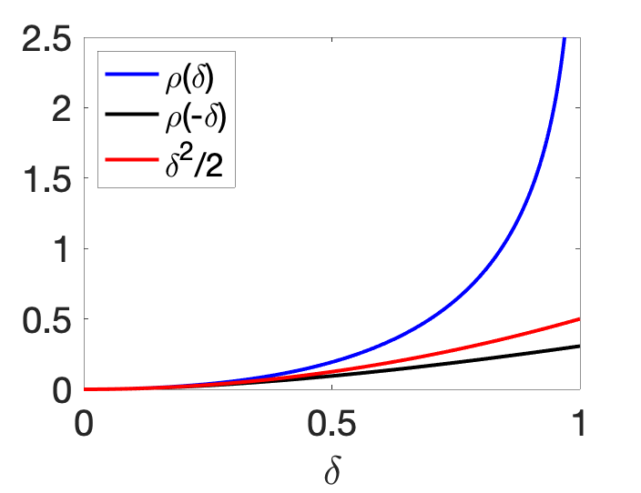
We can then integrate Eq. (3) twice between \(0\) and \(x\) to obtain lower and upper bounds on \(f^\prime\) and then \(f\): $$-f^{\prime\prime}(0)^{1/2} + \frac{f^{\prime\prime}(0)^{1/2}}{1+x f^{\prime\prime}(0)^{1/2}} \leqslant f^\prime(x)-f^\prime(0) \leqslant -f^{\prime\prime}(0)^{1/2} + \frac{f^{\prime\prime}(0)^{1/2}}{1-x f^{\prime\prime}(0)^{1/2}},$$ and $$ \tag{4} \rho \big( – f^{\prime\prime}(0)^{1/2} x \big) \leqslant f(x) \ – f(0) \ – f^\prime(0) x \leqslant \rho \big( f^{\prime\prime}(0)^{1/2} x \big),$$ with \(\displaystyle \rho(u) =\ – \log(1-u) \ – u \sim \frac{u^2}{2} \) when \(u\to 0\), that is, the second-order expansion is tight at \(x =0\), but leads to global lower and upper bounds. This upper-bound is valid as long as \(\delta = f^{\prime\prime}(0)^{1/2} x \in [0,1]\), while the lower-bound on \(f\) is always true. The function \(\rho\) is plotted below.

Properties in multiple dimensions. The properties above in Eq. (3) and (4) directly extend to multiple dimensions. For any \(x \in C\), then for any \(\Delta \in \mathbb{R}^d\) such that \(\delta^2 = \Delta^\top f^{\prime\prime}(x) \Delta < 1\), we have upper and lower bounds for the Hessian, the gradient and the functions value at \(x + \Delta\), that is, denoting by \(\| \cdot \|\) the standard Euclidean norm (see detailed proofs at the end of the post) $$\tag{5}(1-\delta)^2 f^{\prime \prime}(x) \preccurlyeq f^{\prime \prime}(x+\Delta) \preccurlyeq \frac{1}{(1-\delta)^2} f^{\prime \prime}(x),$$ $$ \tag{6}\big\| f^{\prime\prime}(x)^{-1/2} \big(f^\prime(x+\Delta)-f^\prime(x) -f^{\prime \prime}(x)\Delta \big) \big\| \leqslant \frac{\delta^2}{1-\delta},$$ and $$\tag{7} \rho(-\delta) \leqslant f(x+\Delta)\ -f(x) \ – f^\prime(x)^\top \Delta \leqslant \rho(\delta).$$ A nice consequence is that if \(\delta < 1\), then \(x+\Delta \in C\), that is, we get “for free” a feasible point. Moreover, these approximations are “second-order tight” at \(\Delta=0\), that is, the term in \(f^{\prime\prime}(x)\) in Taylor expansion around \(x\) is exact.

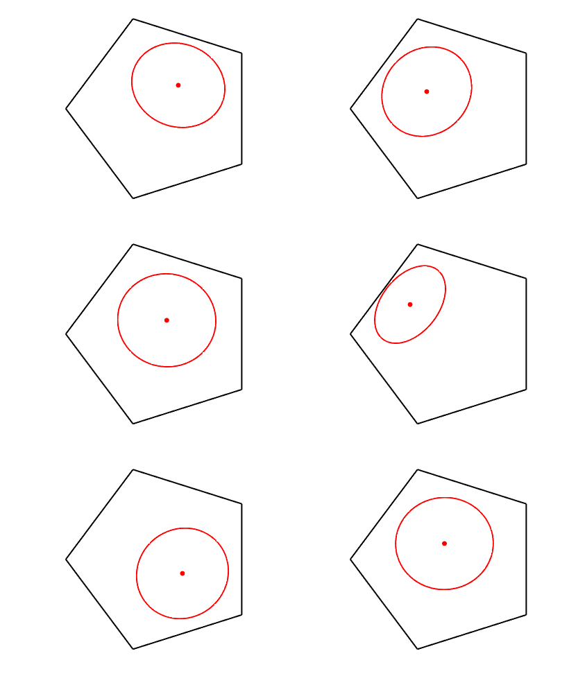
Dikin ellipsoid. The condition that \(\delta^2 = \Delta^\top f^{\prime\prime}(x) \Delta < 1\) defines an ellipsoid around \(x\) which is always strictly inside the domain of \(f\) (see example in the plot below). The results above essentially state that when inside the Dikin ellipsoid, the locally quadratic approximation can be used.

In this post, I will focus primarily on the use self-concordant functions in optimization through the analysis of Newton method.

Why should you care about Newton method?

1. For fun: Newton method is one of the classics of optimization!
2. For high precisions: as we will see, it is quadratically convergent and attains machine precision after solving a few linear systems.
3. Even in high dimensions where the linear system can be expensive, Newton method may still be the method of choice for severely ill-conditioned problems where even accelerated first-order methods are too slow to obtain low precision solutions.
4. It sometimes comes for free in situations where gradients are expensive to evaluate compared to \(d\).

Classical analysis of Newton method

Given a function \(f: \mathbb{R}^d \to \mathbb{R}\), Newton method is an iterative optimization algorithm consisting in locally approximating the function \(f\) around the iterate \(x_{t}\) by a second-order Taylor expansion $$f(x_t) + f^\prime(x_t)^\top(x-x_t) + \frac{1}{2} (x-x_t)^\top f^{\prime \prime}(x_t) ( x – x_t),$$ whose minimum can be found in closed form as $$\tag{8} x_{t+1} = x_t \ – f^{\prime \prime}(x_t)^{-1} f^{\prime}(x_t).$$

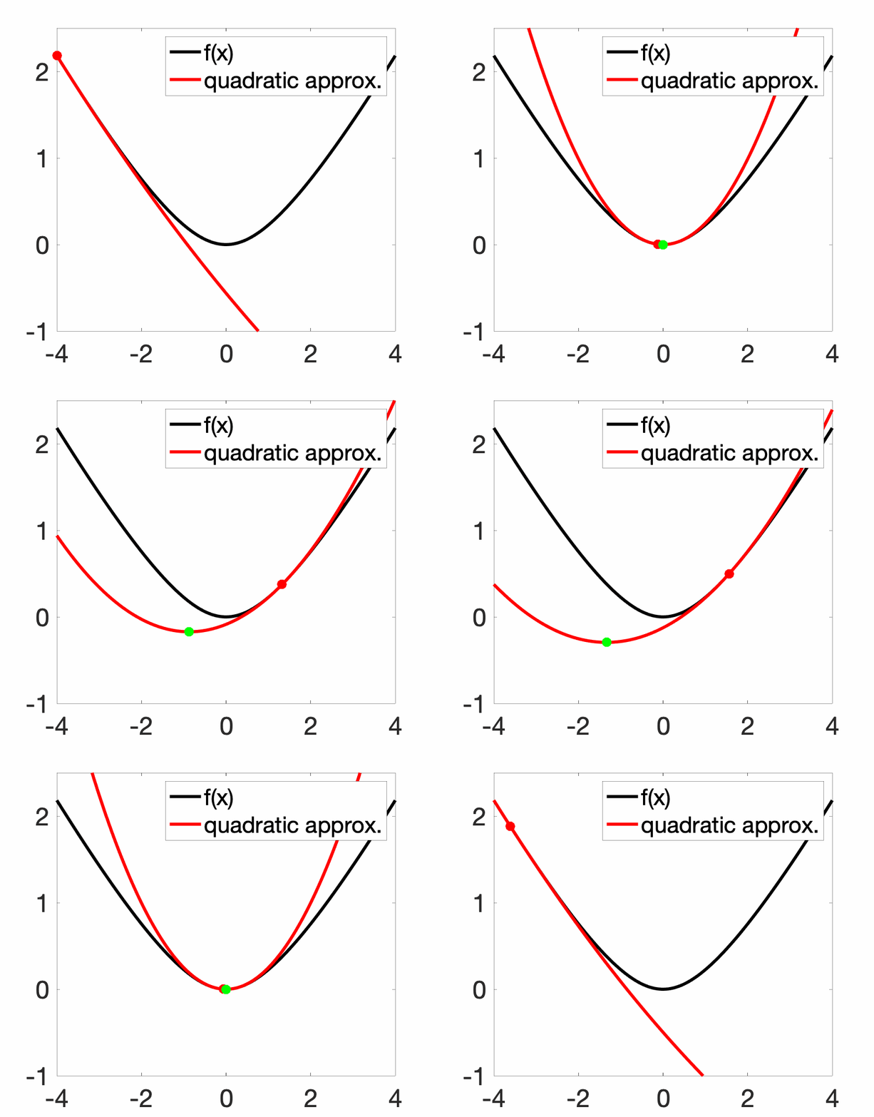
Newton method is classically analyzed for three times differentiable convex functions with bounded Hessians and third-order derivatives. The method is only locally convergent, that is, far away from the global minimizer \(x_\ast\) (even for very regular convex function), the method may diverge. In the non-convex setting, this leads to nice fractal plots, but even for convex functions, the method can be unstable (see plot above).

Locally, it is quadratically convergent, that is, there exists \(c>0\), such that if \(\| x_t \ – x_\ast\| \leqslant c\), then \(\| x_{t+1} \ – x_\ast \| /c \leqslant \big( \|x_t\ – x_\ast\| / c \big)^2\). Roughly, the number of significant digits doubles at every iteration.

This leads to $$ \| x_{t} \ – x_\ast \| \leqslant c \big( \|x_{t_0} \ – x_\ast\| / c \big)^{2^{t-t_0}} ,$$ for \(t \geqslant t_0\) and \(t_0\) an index for which \(\| x_{t_0} \ – x_\ast\| \leqslant c\). It is less than \(\varepsilon\), as soon as \(2^{t-t_0} \log ( c / \| x_{t_0} – x_\ast \| ) \geqslant \log ( c / \varepsilon)\), that is, $$ t \geqslant t_0 + \frac{ \log \log ( c / \varepsilon)}{ \log 2} \ – \frac{\log \log ( c / \| x_{t_0} – x_\ast \| )}{\log 2}.$$

That is, once we enter the quadratic phase, we obtain a number of iterations in \( \log \log ( 1/ \varepsilon)\), that is, only very few iterations. For example, for \(\varepsilon = 10^{-16}\), \(\log \log ( 1/ \varepsilon) \leqslant 4\).

Two major issues may be solved elegantly using self-concordant analysis:

1. Dealing with the two phases of Newton method, the quadratically convergent final phase, as well as the initial phase.
2. Obtaining convergence rates which are affine-invariant, that is, minimizing \(f(x)\) of \(f(Ax+b)\) for \(A\) an invertible matrix should lead to exactly the same convergence rate (this is not the case for the classical analysis, where for example the constant \(c\) depends on non affine-invariant quantities).

Self-concordant analysis of Newton method

Consider \(f: \mathcal{C} \to \mathbb{R}\) which is self-concordant. Since Newton method in Eq. (8) is not globally convergent, we need to study a version where the Newton step is performed partially. There are several possible strategies. Here I present the so-called “damped Newton” iteration and thus study the iteration $$ x^+ = x\ – \frac{1}{1+\lambda(x)} f^{\prime \prime}(x)^{-1} f^\prime(x),$$ where we define the “Newton decrement” \(\lambda(x)\) at \(x \in C\), as $$ \lambda^2 = \lambda(x)^2 =f^\prime(x)^\top f^{\prime \prime}(x)^{-1} f^\prime(x) = \|f^{\prime \prime}(x)^{-1/2} f^\prime(x) \|^2.$$

The Newton decrement is a key quantity in the analysis of Newton method, as \(\frac{1}{2} \lambda(x)^2\) is exactly the decrease in the quadratic approximation obtained by a full Newton step. Moreover,

1. If \(\lambda(x) < 1\), then \(x^+\) is in the Dikin ellipsoid where we can expect the local quadratic approximation to be relevant.
2. If \(\lambda(x) < 1\), then one can show that \(f(x) \ – f(x_\ast) \leqslant \rho( \lambda(x)) \sim \frac{1}{2} \lambda(x)^2\) when \(\lambda(x)\) is close to zero, that is, the Newton decrement provides an upper bound on the distance to optimum.

The update corresponds to \(\Delta = \ – \frac{1}{1+\lambda(x)} f^{\prime \prime}(x)^{-1} f^\prime(x)\), and \(\delta = \frac{\lambda(x)}{1+\lambda(x)} \in [0,1]\), thus \(x^+\) is automatically feasible (which is important for constrained case, see below).

Moreover, using Eq. (7), we get $$f(x^+)-f(x) \leqslant \ – \frac{f^\prime(x)^\top f^{\prime \prime}(x)^{-1} f^\prime(x)}{1+\lambda(x)} + \rho \Big( \frac{\lambda(x)}{1+\lambda(x)} \Big) = \log (1+ \lambda(x)) \ – \lambda(x).$$ This immediately leads to a fixed decrease of \(\frac{1}{4} \, – \log \frac{5}{4} \geqslant 0.0268\) if \(\lambda(x) \geqslant \frac{1}{4}\).

We can now compute the Newton decrement at \(x^+\), to see how it decreases, by first bounding $$\lambda(x^+) =\|f^{\prime \prime}(x^+)^{-1/2} f^\prime(x^+) \| \leqslant \frac{1}{1-\delta} \|f^{\prime \prime}(x)^{-1/2} f^\prime(x^+) \|,$$ using Eq. (5). We then have, using Eq. (6): $$ \|f^{\prime \prime}(x)^{-1/2} f^\prime(x^+) \| \leqslant \big\| f^{\prime \prime}(x)^{-1/2} \big( f^\prime(x) + f^{\prime\prime}(x) \Delta \big) \big\| + \frac{\delta^2}{ 1-\delta } \leqslant \frac{\lambda(x)^2}{1+\lambda(x)} + \frac{\delta^2}{ 1-\delta }.$$ This exactly leads to $$\lambda(x^+) \leqslant 2 \lambda(x)^2, $$ which leads to quadratic convergence if \(\lambda(x)\) is small enough.

We can then divide the analysis in two phases: before \(\lambda(x) \leqslant 1/4\) and after. The first integer \(t_0\) such that \(\lambda(x) \leqslant 1/4\) is less than \(\frac{ f(x_0) – f(x_\ast)}{0.0268} \leqslant 38 [ f(x_0) – f(x_\ast) ]\). Then, for the second phase, \(2\lambda(x_t) \leqslant (1/2)^{2^{t-t_0}}\). Given that for \(\lambda \leqslant 1/4\), \(\rho(\lambda) \leqslant 2\lambda\), we reach precision \(\varepsilon\) as soon as \(2^{t-t_0} \log 2 \geqslant \log \frac{1}{\varepsilon}\), that is, \(t \geqslant t_0 + \frac{1}{\log 2} \log \log \frac{1}{\varepsilon} -1\). This leads to number of iterations to reach a precision \(\varepsilon\) which is less than $$38[ f(x_0) \ – f(x_\ast)] +2 \log \log \frac{1}{\varepsilon}.$$

Interior point methods

Self-concordant functions are also key in the analysis of interior point methods. Consider a function \(f\) defined on \(\mathbb{R}^d\) and the constrained optimization problem $$\min_{ x \in C} f(x),$$ where \(C\) is a convex set. Barrier methods are appending a so-called “barrier function” \(g(x)\) to the objective function. A function \(g\) is a barrier function if \(g\) is convex and with domain containing the relative interior of \(C\), with gradients that explode when reaching the boundary of \(C\). We then solve instead $$\tag{9} \min_{x \in \mathbb{R}^d} \varepsilon^{-1} f(x) + g(x), $$ where \(\varepsilon > 0\). Typically, the minimizer \(x_\varepsilon\) is in the relative interior of \(C\) (hence the name interior point method), and, when \(\varepsilon\) tends to zero, \(x_\varepsilon\) tends to the minimizer of \(f\) on \(C\).

When both the original function \(f\) and the barrier function \(g\) are self-concordant, the (damped) Newton method is particularly useful as it ensures feasibility of the iterates. Moreover, the interplay between the progressive reduction of \(\varepsilon\) towards zero and the approximate resolution of Eq. (9) can be completely characterized (see [3, 4, 5]). This applies directly to linear programming, second-order cone programming and semidefinite programming.

Applications in machine learning

If you have reached this point, you are probably a big fan of self-concordance. While this property is crucial in optimization, is it really relevant for machine learning or statistics? The sad truth is that most of the non-quadratic functions within machine learning are not self-concordant in the sense of Eq. (1) or Eq. (2). In particular, log-sum-exp functions, such that the logistic loss \(f(t) = \log( 1 + \exp(-t) )\), do satisfy a relationship between third and second-order derivatives, but of the form $$| f^{\prime \prime \prime}(t)| \leqslant f^{\prime \prime }(t),$$ without the power \(3/2\). This seemingly small difference leads to several variations [7] which will the topic of next month blog post. Meanwhile, it is worth mentioning two applications in machine learning of classical self-concordance.

Maximum likelihood estimation for covariance matrices. Beyond its use in interior point methods, self-concordant functions arise naturally when estimating the covariance matrix using maximum likelihood estimation with a Gaussian model. Indeed, the negative log-likelihood can be written as $$ – \log p (x| \mu ,\Sigma) =\frac{d}{2} \log(2\pi) + \frac{1}{2} \log \det \Sigma + \frac{1}{2} ( x -\mu)^\top \Sigma^{-1} ( x – \mu),$$ which leads to a negative log-determinant of the inverse \(\Sigma^{-1}\) of the covariance matrix \(\Sigma\), which is a self-concordant function, on which the guarantees discussed above apply.

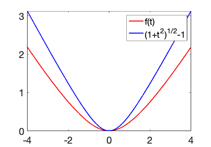
Self-concordant losses. One can also design losses which are self-concordant. For example, a self-concordant version of the Huber loss is $$f(t) = \sqrt{1+t^2} \ – 1 \ – \log \frac{ \sqrt{1+t^2} +1 }{2} .$$ It can be seen as the Fenchel-conjugate of \(– \log(1-t^2)\), and the proximity with a quadratic problem can be leveraged to obtain generalization performances using this loss function which are essentially the same as for the square loss. It can also be used for binary classification (see [8] for details, and the two nice blog posts of Dmitrii Ostrovskii).

One-step-estimation. Given the focus of this post on Newton method, I cannot resist mentioning a great technique coming from statistics that relies on a single Newton step. We consider a classical empirical risk minimization problem (statisticians would call it an M-estimation problem), with empirical risk \(\displaystyle \widehat{R}(\theta) = \frac{1}{n} \sum_{i=1}^n \ell(y_i, f_\theta(x_i) )\). Given an estimator \(\hat{\theta}\), obtained by any means, then if \(\hat{\theta}\) is \(\frac{1}{\sqrt{n}}\) away from the optimal parameter (with optimal performance on unseen data), then one Newton step on the function \(\widehat{R}\) started from \(\hat{\theta}\) will lead to an estimator achieving asymptotically the usual Cramer-Rao lower bound. In a nutshell, a single Newton step on the empirical risk transforms a good estimator into a very good estimator. See [9, Section 5.7] for more details.

Acknowledgements. I would like to thank Adrien Taylor and Dmitrii Ostrovskii for proofreading this blog post and making good clarifying suggestions.

References

[1] F. Bach and E. Moulines. Non-strongly-convex smooth stochastic approximation with convergence rate \(O(1/n)\). Advances in Neural Information Processing Systems (NIPS), 2013.
[2] Andrea Caponnetto, Ernesto De Vito. Optimal rates for the regularized least-squares algorithm. Foundations of Computational Mathematics 7(3):331-368, 2007.
[3] Yurii Nesterov, and Arkadii Nemirovskii. Interior-Point Polynomial Algorithms in Convex Programming, SIAM, 1994.
[4] Arkadii Nemirovski. Interior Point Polynomial Time Methods in Convex Programming. Lecture notes, 1996.
[5] Yurii Nesterov. Lectures on Convex Optimization (Vol. 137). Springer, 2018.
[6] Stephen P. Boyd, and Lieven Vandenberghe. Convex Optimization. Cambridge University Press, 2004.
[7] Francis Bach. Self-Concordant Analysis for Logistic Regression. Electronic Journal of Statistics, 4, 384-414, 2010
[8] Dmitrii Ostrovskii, and Francis Bach. Finite-sample Analysis of M-estimators using Self-concordance. Electronic Journal of Statistics, 15(1):326-391, 2021.
[9] Aad W. Van der Vaart. Asymptotic Statistics, volume 3. Cambridge University Press, 2000.

Detailed proofs for self-concordance properties

We first show Eq. (7), by considering the function \(a(t) = f(x+t\Delta)\), which is a one-dimensional self-concordant function, for which \(a^\prime(t) = \Delta^\top f^\prime(x+t\Delta)\), and \(a^{\prime\prime}(t) = \Delta^\top f^{\prime\prime}(x+t\Delta) \Delta\). Then \(a^{\prime\prime}(0) = \delta^2\), and Eq. (4) for \(x=1\) and \(a\) exactly leads to Eq. (7).

In order to show Eq. (5), we consider \(h \in \mathbb{R}^d\), and the function \(b(t) = h^\top f^{\prime\prime}(x+t\Delta) h\). We have, \(b'(t) = f^{\prime\prime\prime}(x+t\Delta)[h,h,\Delta]\), which can be bounded using Eq. (2) as $$ |b'(t) | \leqslant 2 f^{\prime\prime}(x+t\Delta)[h,h] f^{\prime\prime}(x+t\Delta)[\Delta,\Delta]^{1/2} = 2 b(t) a^{\prime \prime}(t)^{1/2} \leqslant 2 b(t) \frac{\delta}{1-t\delta}, $$ using Eq. (3). This implies that for \(\delta t \in [0,1)\): $$\frac{d}{dt} \big[ (1-\delta t)^2 b(t) \big] = -2\delta (1-\delta t) b(t) + (1-\delta t)^2 b'(t) \leqslant 0, $$ which implies \(b(t) \leqslant \frac{b(0)}{(1-\delta t)^2} = \frac{h^\top f^{\prime\prime}(x) h}{(1-\delta t)^2}\), which leads to the right-hand side of Eq. (5) since this is true for all \(h \in \mathbb{R}^d\). The left-hand side is proved similarly.

In order to show Eq. (6), we consider the function \(g(t) = h^\top f^\prime(x+t\Delta)\), for which, \(g^\prime(t) = h^\top f^{\prime\prime}(x+t\Delta) \Delta\), and \(g^{\prime\prime}(t) = f^{\prime\prime\prime}(x+t\Delta) [h,\Delta,\Delta]\), which satisfies: $$|g^{\prime\prime}(t)| \leqslant 2 f^{\prime\prime}(x+t\Delta)[\Delta,\Delta] f^{\prime\prime}(x+t\Delta)[h,h]^{1/2} \leqslant 2 b(t)^{1/2} a^{\prime \prime}(t). $$ This leads to $$ |g^{\prime\prime}(t)| \leqslant 2 \big( h^\top f^{\prime\prime}(x) h\big)^{1/2} \frac{\delta^2}{(1-\delta t)^3}.$$ We can then integrate twice, using \(g(0) = h^\top f^\prime(x)\) and \(g^\prime(0) = h^\top f^{\prime\prime}(x) \Delta\), to get: $$h^\top \big(f^\prime(x+t\Delta)-f^\prime(x) \ – f^{\prime \prime}(x)\Delta \big) \leqslant \big( h^\top f^{\prime\prime}(x) h\big)^{1/2} \frac{\delta^2}{1-\delta},$$ which leads to Eq. (5) after maximizing with respect to \(h\).