The “η-trick” or the effectiveness of reweighted least-squares

Optimizing a quadratic function is often considered “easy” as it is equivalent to solving a linear system, for which many algorithms exist. Thus, reformulating a non-quadratic optimization problem into a sequence of quadratic problems is a natural idea.

While the standard generic way is Newton method, which is adapted to smooth (at least twice-differentiable) functions, another quite generic way is to use what I have been calling within my lab the “η-trick”.

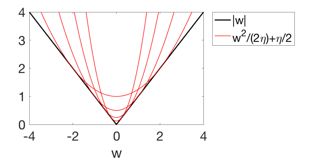
This can be applied to non-smooth functions, and the simplest version is based on this simple identity: $$ |w| = \min_{ \eta \geq 0 } \frac{1}{2} \frac{w^2}{\eta} + \frac{1}{2} \eta, $$ with the optimal \(\eta\) being equal to \(|w|\) (a simple proof comes from “completing the square”, \(\frac{1}{2} \frac{w^2}{\eta} + \frac{1}{2} \eta = \frac{1}{2} \frac{(|w| – \eta)^2}{\eta} + |w|\), for another proof, simply differentiate with respect to \(\eta\)).

We thus obtain a variational formulation of \(|w|\) as the minimum over \(\eta\) of a quadratic function in \(w\), as shown below for four values of \(\eta\).

Application to Lasso / basis pursuit

The most classical application is the Lasso problem (as proposed in [3, 4]): $$\min_{w \in \mathbb{R}^d} \frac{1}{2n} \| y – X w \|_2^2 + \lambda \| w\|_1,$$ where \(X \in \mathbb{R}^{n \times d}\) is the design matrix (input variables), \(y \in \mathbb{R}^n\) the vector of responses (output variable), \(\| \cdot \|_2\) the \(\ell_2\)-norm defined through \(\|z\|_2^2 = \sum_{j=1}^d z_j^2\), and \(\|w\|_1 = \sum_{j=1}^d |w_j|\) is the \(\ell_1\)-norm, which is known to be “sparsity-inducing” (that is, it leads to many zero values in the minimizer \(w\) if \(\lambda\) is large enough).

With the variational formulation above applied to each \(w_j\), we get $$ \min_{w \in \mathbb{R}^d} \frac{1}{2n} \| y – X w \|_2^2 + \lambda \| w\|_1 = \min_{w \in \mathbb{R}^d} \min_{\eta \in \mathbb{R}_+^d} \frac{1}{2n} \| y – X w \|_2^2 + \frac{\lambda}{2} \sum_{j=1}^d \frac{w_j^2}{\eta_j} + \frac{\lambda}{2} \sum_{j=1}^d \eta_j.$$

The key aspect of the variational formulation as a minimization problem is that we obtain a joint minimization problem in the variables \((w,\eta)\), for which we can consider alternating optimization (i.e., alternating between minimizing with respect to \(w\) and minimizing with respect to \(\eta\)). The optimum with respect to \(\eta\) is obtained as \(\eta_j = |w_j|\), and the optimization with respect to \(w\) is also simple because of the overall linear/quadratic dependence. The gradient with respect to \(w\) is equal to $$ \frac{1}{n}X^\top ( X w – y ) + \lambda{\rm Diag}(\eta)^{-1} w ,$$ and thus the zero gradient solution can be obtained by solving the linear system \(\big( \frac{1}{n} X^\top X + \lambda {\rm Diag}(\eta)^{-1} \big) w = \frac{1}{n} X^\top y\). This leads to a two-line (in Python or Matlab) algorithm for solving the Lasso problem. For more details on avoiding convergence issues around zero values of \(\eta\) or \(w\), and on solving the linear system efficiently and robustly, see the two monographs [1, Section 5] and [2, Section 5.4].

Another nice aspect of the variational formulation above is that it is jointly convex in \((w,\eta),\) and hence traditional optimization algorithms are globally convergent.

This formulation as a “min-min” problem should be contrasted with the classical variational formulation of the \(\ell_1\)-norm as a maximum, that is, \(\|w\|_1 = \max_{ \|s\|_\infty \leq 1} w^\top s\), which would lead to a “min-max” problem (which leads also to a suite of interpretations and algorithms, but this is for another post).

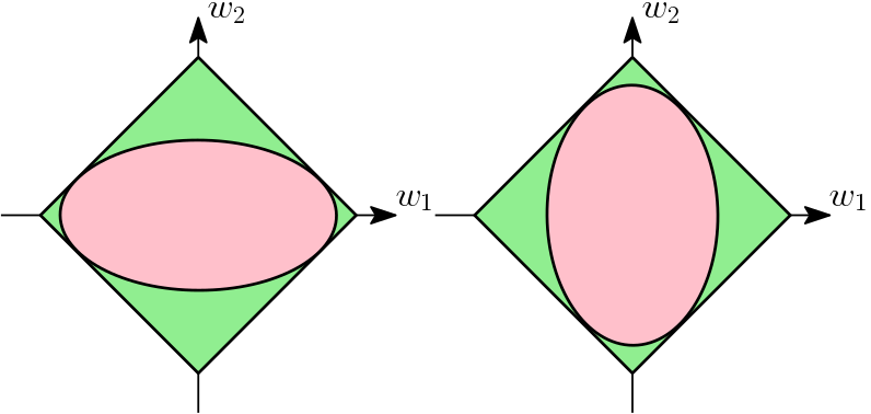
There is another classical formulation for the squared \(\ell_1\)-norm through $$ \| w\|_1^2 =\min_{ \eta \in \Delta_d} \sum_{j=1}^d \frac{w_j^2}{\eta_j},$$ where \(\Delta_d = \{ \eta \in \mathbb{R}_+^d, \ \sum_{j=1}^d \eta_j = 1\}\) is the simplex in \(\mathbb{R}^d\). Thus the squared \(\ell_1\)-norm is the minimum of squared weighted \(\ell_2\)-norms. This leads to the simple geometric interpretation (below in two dimensions).

While the η-trick is most easy for the \(\ell_1\)-norm, it applies to many other situations which I describe below.

Extension to “subquadratic” norms

Given the representation of the \(\ell_1\)-norm as a quadratic function, one may wonder if this can be extended to other norms. In order to preserve the homogeneity of a norm \(\Omega\) defined on \(\mathbb{R}^d\), a natural generalization is a representation in the form $$\Omega(w) = \min_{ \eta \in \mathbb{R}_+^d} \frac{1}{2} \sum_{j=1}^d \frac{w_j^2}{\eta_j} + \frac{1}{2} f(\eta),$$ where \(f\) is convex and \(1\)-homogeneous (then a constrained optimization formulation for \(\Omega(w)^2\) can then also be derived, with the simplex replaced by a level set of \(f\)).

Given that a minimum of linear functions is concave, we see that a necessary condition for the existence of such a parameterization is that \(\Omega(w)\) is a concave function of \(w \circ w = (w_1^2,\dots,w_d^2)\). It turns out that this is also a sufficient condition, and that the function \(f\) can be obtained from \(\Omega\) using Fenchel conjugacy (see [1, Section 1.4.2]).

Examples include various group norms of the forms \(\Omega(w) = \sum_{G \in \mathcal{G}} \| w_G \|_2\), where \(\mathcal{G}\) is a set of subsets of \(\{1,\dots,d\}\) and \(\| w_G\|_2\) is the \(\ell_2\)-norm of the subvector \(w_G\) obtained from \(w\) by only keeping the components whose indices are in \(G\) (this form of “group penalty” is common in structured sparsity [1, Section 1.3] where one wants to force of lot of zeros in \(w\), but also wants to encourage some specific patterns in the set of non-zero components). Thus, for all of these, one can derive simple estimation algorithms with a sequence of least-squares problems (there is another connection with multiple kernel learning [1, Section 1.5], see future posts).

Extensions to all norms

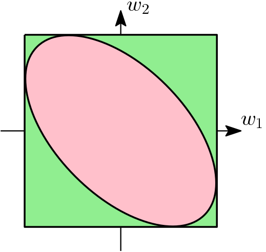
This trick can in fact be extended to all norms, but this requires a non-diagonal Hessian for the quadratic term, where \({\rm Diag}(\eta)\) now becomes a symmetric positive semi-definite matrix \(\Lambda\): $$\Omega(w) = \min_{ \Lambda \in \mathbb{R}^{d \times d} } \frac{1}{2} w^\top \Lambda^{-1} w + \frac{1}{2} g(\Lambda),$$ see [1, Section 5.2] for more details, where an explicit candidate for the function \(g(\Lambda)\) is given. Here, we impose that \(g(\Lambda)\) is infinite when \(\Lambda\) is not positive semi-definite (to make the quadratic function in \(w\) convex).

For example, for the \(\ell_\infty\)-ball below, the ellipsoid has axes which are not parallel anymore to the coordinate axes).

We can also consider the total variation penalty of the form \( \Omega(w) = \sum_{i,j} d_{ij} |w_i – w_j|,\) where the \(d_{ij}\)’s are positive weights. It is commonly used to encourage piecewise constant vectors \(w\). The η-trick can be applied to all terms \(|w_i – w_j|\) [7]. This leads to algorithms solving Laplacian systems for which particularly efficient randomized methods are available (see, e.g., [8]).

Extension to spectral norms

When dealing with a spectral norm on a matrix \(W \in \mathbb{R}^{n \times d}\), that is a norm that depends only on the singular values of \(W\), then one has a specific representation. For example, for the nuclear norm \(\| W\|_\ast\), which is equal to the sum of singular values of \(W\) and encourages matrices with low-rank: $$\| W\|_\ast = \min_{ \Lambda \in \mathbb{R}^{d \times d}} \frac{1}{2} {\rm tr} \big( W \Lambda^{-1} W^\top \big) + \frac{1}{2} { \rm tr} \Lambda,$$ with the constraint that \(\Lambda\) is symmetric positive semi-definite. This leads to simple least-squares based algorithms for nuclear norm minimization [5].

Extensions to non-convex penalties

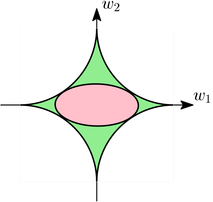
As mentioned above, a necessary condition for a variational representation of a function \(w \mapsto \varphi(w)\) as a minimum of quadratic functions with diagonal Hessians is the concavity in \(w \circ w\) (the vector composed of squares of the components of \(w\)). Other functions beyond norms or squared norms can be considered, such as the following non-convex penalty: $$\frac{1}{\alpha} \| w\|_\alpha^\alpha = \inf_{\eta \in \mathbb{R}_+^d} \frac{1}{2} \sum_{j=1}^d \frac{w_j^2}{\eta_j } + \frac{1}{2\beta } \| \eta \|_\beta^\beta, $$ where for any \(\gamma >0\), \(\| w\|_\gamma^\gamma = \sum_{j=1}^d |w_j|^\gamma\), \(\alpha \in (0,2)\) and \(\beta = \frac{\alpha}{2-\alpha} >0 \). These penalties are commonly used to enhance the sparsity-inducing effect of the \(\ell_1\)-norm or more generally all sparsity-inducing norms: by being non convex penalties (when \(\alpha \in (0,1)\)), they can be more aggressive in setting components of \(w\) to zero (as can be seen below through the “corners” of the corresponding ball being more “pointy”).

The minimizer \(\eta\) above can be obtained in closed form as \(\eta_j = |w_j |^{2-\alpha}\), and thus the same alternating optimization algorithm can be used. Moreover, the geometric interpretation in terms of enclosing ellipsoids for level sets of \(\| w\|_\alpha\) still holds but this is not anymore a convex set. See below for the unit ball of \(\| \cdot \|_{1/2}\).

This leads to reweighted least-squares algorithms when using those penalties, again based on alternating minimization with respect to \(w\) and \(\eta\) [4, 6]. A key difference with the convex case is that the optimization problem is not jointly convex in \((w,\eta)\) anymore, and it typically only converges to a local optimum. Note here that reweighted-\(\ell_1\) algorithms (that use a sequence of weighted \(\ell_1\)-regularized problems) are also commonly used, see [2, Section 5.3].

Beyond regularization penalties

While I focused primarily on regularizers, can we apply this to the loss as well? Using the same recipe, “concavity in the squared arguments”, we get naturally new representations, which can be used in particular for optimization purposes.

A notable one is for the logistic function \(\varphi(u) = \log(1+e^{-u})\) used within logistic regression, which can be written as \(\varphi(u) = -\frac{u}{2} + \log( e^{u/2} + e^{-u/2})\), with the function \(u \mapsto \log( e^{u/2} + e^{-u/2})\) being convex in \(u^2\) (which can be shown by computing the second-order derivative). This leads to the representation [9] $$ \log( e^{u/2} + e^{-u/2}) = \min_{v \in \mathbb{R}}\ \ \log( e^{v/2} + e^{-v/2}) + \frac{ \tanh \frac{v}{2}}{4v} ( u^2 – v^2 ),$$ which is a quadratic variational representation that could be used to optimize the logistic regression objective function (in particular within surrogate function methods commonly used for online dictionary learning, see [10]) or for variational inference [9] (note here that the joint convexity in \(u\) and the inverse of the parameter of the quadratic function is gone).

As shown below, the quadratic upper-bound can be contrasted with (a) the second-order Taylor expansion (thus with matching first two derivatives), which is not an upper-bound (and thus may not lead to global convergence when used for optimization, that is, when Newton method is used), and (b) the upper-bound obtained from the uniform bound \(1/4\) on the second-derivative, which is weaker in particular for large values of \(u\) (and corresponds to using the traditional notion of smoothness of the objective function).

Now, you can go ahead and use the η-trick within your optimization problems. But it goes beyond and it pops out in other areas in machine learning, in particular for multiple kernel learning, super-Gaussian distributions and convex relaxations of combinatorial penalties. These will be the topics of future posts.

References

[1] Francis Bach, Rodolphe Jenatton, Julien Mairal, Guillaume Obozinski. Optimization with sparsity-inducing penalties. Foundations and Trends in Machine Learning, 4(1):1-106, 2012. 
[2] Julien Mairal, Francis Bach, Jean Ponce. Sparse Modeling for Image and Vision Processing. Foundations and Trends in Computer Vision, 8(2-3):85-283, 2014.
[3] Yves Grandvalet and Stéphane Canu. Outcomes of the equivalence of adaptive ridge with least absolute shrinkage. Advances in Neural Information Processing Systems (NIPS), 1999.
[4] Ingrid Daubechies, Ronald DeVore, Massimo Fornasier, and C. Sinan Güntürk. Iteratively reweighted least squares minimization for sparse recovery. Communications on Pure and Applied Mathematics, 63(1):1–38, 2010.
[5] Andreas Argyriou, Theodoros Evgeniou, and Massimiliano Pontil. Multi-task feature learning. Advances in Neural Information Processing Systems (NIPS), 2007.
[6] Rodolphe Jenatton, Guillaume Obozinski, and Francis Bach. Structured sparse principal component analysis. Proceedings of the International Conference on Artificial Intelligence and Statistics (AISTATS), 2010.
[7] Philipp Grohs, and Markus Sprecher. Total variation regularization on Riemannian manifolds by iteratively reweighted minimization. Information and Inference, 4: 353-378, 2016.
[8] Rasmus Kyng, and Sushant Sachdeva. Approximate Gaussian elimination for Laplacians-fast, sparse, and simple. Annual Symposium on Foundations of Computer Science (FOCS), 2016.
[9] Tommi S. Jaakkola and Michael I. Jordan. Bayesian parameter estimation via variational methods. Statistics and Computing, 10(1):25-37, 2000.
[10] Julien Mairal, Francis Bach, Jean Ponce, and Guillermo Sapiro. Online learning for matrix factorization and sparse coding. Journal of Machine Learning Research, 11:10-60, 2010.