The Gumbel trick

Quantities of the form \(\displaystyle \log \Big( \sum_{i=1}^n \exp( x_i) \Big)\) for \(x \in \mathbb{R}^n\), often referred to as “log-sum-exp” functions are ubiquitous in machine learning, as they appear in normalizing constants of exponential families, and thus in many supervised learning formulations such as softmax regression, but also more generally in (Bayesian or frequentist) probabilistic modelling. Moreover, as often used in optimization, they are a standard way of performing a soft maximum. In this context, the function defined as $$ \displaystyle f_\varepsilon(x) = \varepsilon \log \Big( \sum_{i=1}^n \exp( x_i / \varepsilon) \Big),$$ is such that \( \displaystyle \lim_{\varepsilon \to 0^+} f_\varepsilon(x) = \max\{x_1,\dots,x_n\}\).

Is it possible to go from the maximum back to the softmax \(f_\varepsilon(x)\) (for any strictly positive \(\varepsilon\), and thus equivalently for \(\varepsilon=1\)) ? Beyond being a nice mathematical puzzle, this would be useful for very large \(n\) when the maximization problem could be easier than the summation problem (more on this below).

While this seems at first impossible, the Gumbel trick provides a surprising randomized solution. We consider adding some independent and identically distributed random variables \(\gamma_1,\dots,\gamma_n\), to form the vector \(x + \gamma \in \mathbb{R}^n\) and takes its maximum component, that is, $$
y = x + \gamma \mbox{ and } z = \max \big\{ y_1,\dots, y_n \big\} = \max \big\{ x_1 + \gamma_1,\dots,x_n +\gamma_n \big\}.$$ With a well chosen distribution for the components of \(\gamma\), we exactly have $$\mathbb{E} z =
\mathbb{E} \max \big\{ y_1,\dots, y_n \big\} = \mathbb{E} \max \big\{ x_1 + \gamma_1,\dots,x_n +\gamma_n \big\} = \log \Big( \sum_{i=1}^n \exp( x_i) \Big).$$ This is achieved by the Gumbel distribution, hence the name “Gumbel trick” (the first applications within machine learning seem to be from [1] and [2], while this is a well-known fact in social sciences, see, e.g., [3]). We first make a detour through exponential distributions.

Minimum of independent exponential distributions

A random variable \(T\) is distributed according to the exponential distribution with parameter \(\lambda \in \mathbb{R}\), if it is supported on the positive real line and its density there is equal to \(t \mapsto \lambda \exp( – \lambda t).\) We have these classical properties:

• \(\mathbb{E} T = 1/\lambda\) and \({\rm var}(T) = 1/ \lambda^2\).
• \(T\) has the same distribution as \(-( 1/\lambda)\log U\), where \(U\) has a uniform distribution on \([0,1]\), leading to a simple algorithm to sample \(T\).

A key property which is used heavily in point processes and queuing theory is characterizing the minimum and minimizer of independent exponentially distributed random variables.

Proposition. Given \(n\) independent variables \(T_i\) distributed according to exponential distributions with parameter \(\lambda_i\), \(i=1,\dots,n\), the minimum \(V = \min \{T_1,\dots,T_n\}\) is distributed according to an exponential distribution with parameter \(\lambda_1+\dots+\lambda_n\), and the minimizer \(i^\ast= \arg \min_{i \in \{1,\dots,n\}} T_i\) (breaking ties arbitrarily) is distributed according to a multinomial distribution of parameter \(\pi\) with \(\displaystyle \pi_i = \frac{\lambda_i}{ \lambda_1 + \cdots + \lambda_n}\), for \(i \in \{1,\dots,n\}\). Moreover, \(i^\ast\) and \(V\) are independent.

(simple) Proof. A direct integration shows that $$ \mathbb{P}( T \geq u) = \int_{u}^{+\infty} \lambda \exp( -\lambda t) = \exp(-\lambda u).$$ We can then directly compute the probability, for a fixed \(i \in {1,\dots,n}\) and \(u \in \mathbb{R}_+\): $$
\mathbb{P}( I^\ast = i, V \geq u) = \mathbb{P}( T_i \geq u, \forall j \neq i, T_j \geq T_i),$$ which is equal by independence of all \(T_j\)’s to $$ \int_{u}^{+\infty} \Big( \prod_{ j\neq i} \exp( – \lambda_j t_i) \Big) \lambda_i \exp( – \lambda_i t_i) dt_i = \exp\Big( – u \sum_{i=1}^n \lambda_i \Big) \times \frac{\lambda_i}{ \lambda_1 + \cdots + \lambda_n},$$ which exactly shows the desired result (both independence and the claimed distributions).

From exponential to Gumbel distributions

A real random variable \(\Gamma\) is distributed according to a Gumbel distribution with parameter \(x \in \mathbb{R}\), if it is equal in distribution to \(\Gamma = -\log T – C\), where \(T\) is distributed according to an exponential distribution of parameter \(\lambda = \exp(x)\), and \(C\approx 0.5772\) is the Euler constant (note that in some conventions, \(C\) is not subtracted). We have the following properties:

• \(\mathbb{E} \Gamma = x\) where Indeed, we have: $$ \mathbb{E} \Gamma= -\int_0^{+\infty} \log (y\exp(-x)) \exp(-y) dy\ – C= x \ – \int_0^{+\infty} (\log y)\exp(-y) dy \ – C = x,$$ with a standard property of the Euler constant.
• \({\rm var}(\Gamma) = \frac{\pi^2}{6}\) (proof left as an exercise, derivatives of the Gamma function could be handy).
• \(\Gamma\) has the same distribution as \(x – C – \log( – \log U) \), where \(U\) has a uniform distribution on \([0,1]\), leading to a simple algorithm to sample \(\Gamma\).
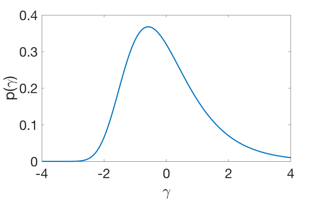
• The density of \(\Gamma\) is \(p(\gamma) = \exp( x-\gamma -C – \exp( x – \gamma – C) )\), as shown below for \(x=0\).

The proposition above on exponential distributions leads to the following result.

Proposition. Given \(n\) independent variables \(\Gamma_i\) distributed according to Gumbel distributions with parameter \(x_i\), \(i=1,\dots,n\), the maximum \(Z = \max \{\Gamma_1,\dots,\Gamma_n\}\) is distributed according to a Gumbel distribution with parameter (and thus mean) \(\log \big( \sum_{k=1}^n \exp(x_k) \big)\), the minimizer \(i^\ast= \arg \max_{i \in {1,\dots,n}} \Gamma_i\) (breaking ties arbitrarily) is distributed according to a multinomial distribution of parameter \(\pi\) with \(\displaystyle \pi_i = \frac{\exp(x_i)}{ \exp(x_1) + \cdots + \exp(x_n)}\), for \(i \in {1,\dots,n}\). Moreover, \(i^\ast\) and \(Z\) are independent.

Applications in machine learning

The Gumbel trick can be used in mainly two ways: (a) the main goal is to approximate the expectation using a finite average or using stochastic gradients (then only the value of the maximum is used), (b) the minimizer is used for sampling purposes. I will focus only on the first type of applications and refer to the very nice posts of Tim Vieira, Chris Maddison, and Laurent Dinh for the sampling aspects.

Log-partition functions

We consider \(d\) finite sets \(\mathcal{X}_1,\dots,\mathcal{X}_d\), and a probability mass function at \(x = (x_1,\dots,x_d)\) of the form: $$p(x) = p(x_1,\dots,x_d) = \exp( f(x)\ – A(f)),$$ where \(f: \mathcal{X}_1 \times \dots \times \mathcal{X}_d \to \mathbb{R}\) is a any function, and $$ A(f) = \log \big( \sum_{x_1 \in \mathcal{X}_1,\dots,x_d \in \mathcal{X}_d} \exp( f(x) ) \big)$$ is the so-called log-partition function (which is here to make the probability mass sum to one). The cardinality of \(\mathcal{X}_1 \times \dots \times \mathcal{X}_d\) is exponential in \(d\) and thus the sum defining \(A(f)\) cannot in general be computed even for moderate \(d\). Since computing \(A(f)\) or its derivatives is a key step in many inference tasks, finding approximations is one of the standard computational problems in probabilistic modelling.

The Gumbel trick allows to go from maximization problems to “log-sum-exp” problems, and is only useful when the maximization problem is easy to solve while the “log-sum-exp” problem is not. Can this really happen? In other words…

Is the Gumbel trick useful?

There are many conditions under which combinatorial optimization problems can be solved in polynomial time, but two properties have emerged as crucial (at least in machine learning applications): (1) dynamic programming, and (2) linear programming. For simplicity, I will illustrate them for binary problems where \(\mathcal{X}_i = \{0,1\}\) for all \(i\), and so-called “cut functions” \(f(x) = \sum_{i,j = 1}^d w_{i,j} x_i x_j + \sum_{i=1}^d w_i x_i\), for arbitrary scalar weights \(w_{i,j}\), \(w_i\).

• Dynamic programming: this corresponds to the situations where most of the weights \(w_{i,j}\) are equal to zero, with the graph on the vertex set \(\{1,\dots,n\}\) with edge set equal to the pairs \((i,j)\) with \(w_{i,j}\neq 0\), being a tree, or a chain.
  For example, consider \(f(x) = \sum_{i=1}^{d-1} w_{i,i+1} x_i x_{i+1} + \sum_{i=1}^d w_i x_i\). In this situation, one can compute sequentially the functions (with increasing index \(k\)) $$ f_k(x_k) = \max_{x_1,\dots,x_{k-1}} \sum_{i=1}^{k-1} w_{i,i+1} x_i x_{i+1} + \sum_{i=1}^k w_i x_i,$$ noticing that $$f_{k+1}(x_{k+1}) = \max_{x_{k} \in \{0,1\}} f_k(x_k) + w_{k-1,k} x_k x_{k+1} + w_{k+1} x_{k+1}, $$ which can be computed easily; the recursion leads to the desired value \(\max_{x_{d} \in \{0,1\}} f_d(x_d)\).
  In order to obtain the identity above, we have simply used the property $$\max\{ A + B, C + B\} = B + \max \{A,C\}.$$ However, this property is also true for the softmax, as $$\log \big( \exp(A + B) + \exp(C + B) \big) = B+ \log \big( \exp(A) + \exp(C ) \big).$$ Thus, the same dynamic programming strategy works for softmax, and using the Gumbel trick is here useless. (here, we have described a particular instance of the sum-product and max-product algorithms for graphical models).

• Linear programming: for the particular generic quadratic binary problem, we can write for any \(x_i,x_j \in \{0,1\}\), \(x_i x_j = \min \{x_i,x_j\}\), and, if all \(w_{i,j}\) are non-positive (and here no constraint regarding having many zero values), then the function \(g: \mathbb{R}^d \to \mathbb{R}\) defined as \(g(x) = \sum_{i,j = 1}^d w_{i,j} \min \{x_i,x_j\} + \sum_{i=1}^d w_i x_i\) is concave and equal to \(f\) for \(x \in \{0,1\}^d\). The convex relaxation of computing \(\max_{x \in \{0,1\}^d} f(x)\) is \(\max_{x \in [0,1]^d} f(x)\), which is a concave maximization problem, which can be solved in polynomial time (it can be cast as a linear programming problem). For this particular problems, due to a property called submodularity, the convex relaxation happens to be tight. In these situations, maximizing is feasible while “log-sum-exp” is not. However, the Gumbel trick requires to perturb \(f(x)\) with a different random values for all \(2^d\) assignments of \((x_1,\dots,x_d)\), thus totally losing the structure above. Therefore, using the Gumbel trick is here also useless.

Thus it seems that for classical situations where maximization can be done in polynomial time, the Gumbel trick is useless, either because performing log-sum-exp is as simple (for dynamic programming), or because maximization is intractable once the Gumbel perturbations are added (for linear programming). Can we make it useful?

Separable Gumbel perturbations

This is where Tamir Hazan and Tommi Jaakkola [4] come in with the following very nice and important result, which is true beyond cut functions, and shows that with a separable random perturbation, we get an upper-bound of the log-partition function.

Proposition. Given \(d\) random functions \(\gamma_i : \mathcal{X}_i \mapsto \mathbb{R}\), \(i=1,\dots,d\), such that each value (within and across the functions) is sampled independently distributed from a Gumbel distribution with zero mean, then $$A(f) \leq \mathbb{E} \Big[ \max_{x_1 \in \mathcal{X}_1,\dots,x_d \in \mathcal{X}_d} f(x) + \sum_{i=1}^d \gamma_i(x_i)\Big].$$

Proof. We can show the result by induction on \(d\), by first conditioning on \(\gamma_d\) to get $$\mathbb{E} \Big[ \! \max_{x_1,\dots,x_d} \!f(x_1,\dots,x_d) + \! \sum_{i=1}^d \gamma_i(x_i)\Big] = \mathbb{E} \bigg[\mathbb{E} \Big[ \! \max_{x_1,\dots,x_d} \!f(x_1,\dots,x_d) + \! \sum_{i=1}^d \gamma_i(x_i) \ \Big| \ \gamma_d \Big] \bigg], $$ and the property that the expectation of the max is larger than the max of the expectation to get the lower-bound $$ \mathbb{E} \bigg[ \max_{x_d} \mathbb{E} \Big[ \! \max_{x_1,\dots,x_{d-1}} \!f(x_1,\dots,x_d) + \! \sum_{i=1}^d \gamma_i(x_i) \ \Big| \ \gamma_d \Big] \bigg].$$ It is equal to $$ \mathbb{E} \bigg[ \max_{x_d} \Big\{ \gamma_{d}(x_d) + \mathbb{E} \Big[ \! \max_{x_1,\dots,x_{d-1}} \!f(x_1,\dots,x_d) + \! \sum_{i=1}^{d-1} \gamma_i(x_i) \ \Big| \ \gamma_d \Big] \Big\} \bigg], $$ which is lower-bounded by applying the result for \(d-1\), by $$ \mathbb{E} \max_{x_d} \Big\{ \gamma_d(x_d) + \log \Big( \sum_{x_1 ,\dots,x_{d-1}} \exp(f(x))\Big) \Big\} = \log \Big( \sum_{x_1 ,\dots,x_{d}} \exp(f(x))\Big),$$ by applying the regular Gumbel trick to \(\gamma_d\).

For binary problems like for cut-functions, this corresponds to adding to \(f(x) = \sum_{i,j = 1}^d w_{i,j} x_i x_j + \sum_{i=1}^d w_i x_i\), the term \(\sum_{i=1}^d x_i \gamma_i(1) + \sum_{i=1}^d (1-x_i) \gamma_i(0)\), which is a linear function of \(x\), and still leading to a tight convex relaxation. Here \(2d\) Gumbel variables are used instead of \(2^d\).

This seminal result led to a series of works using this result to approximate the log-partition function for parameter learning in intractable distributions where the maximization problem is efficient [5, 6].

Interestingly, the Gumbel trick is a simple consequence of a special property of a specific exponential family (here the exponential distribution). Some other exponential families (e.g., Gamma or Dirichlet) lead to different special properties with other nice consequences, but this is for future posts.

References

[1] Dima Kuzmin and Manfred K. Warmuth. Optimum follow the leader algorithm. Proceedings of the Conference on Learning Theory (COLT), 2005.
[2] George Papandreou, Allan L. Yuille. Perturb-and-MAP random fields: Using discrete optimization to learn and sample from energy models. Proceedings of the International Conference on Computer Vision (ICCV), 2011.
[3] John I. Yellott Jr. The relationship between Luce’s choice axiom, Thurstone’s theory of comparative judgment, and the double exponential distribution. Journal of Mathematical Psychology, 15.2: 109-144. 1977.
[4] Tamir Hazan and Tommi Jaakkola. On the Partition Function and Random Maximum A-Posteriori Perturbations. Proceedings of the International Conference on Machine Learning (ICML) , 2012.
[5] Andreea Gane, Tamir Hazan, and Tommi Jaakkola. Learning with maximum a-posteriori perturbation models. Proceedings of the Conference on Artificial Intelligence and Statistics (AISTATS), 2014.
[6] Tatiana Shpakova and Francis Bach. Parameter Learning for Log-supermodular Distributions. Advances in Neural Information Processing Systems (NIPS), 2016.