Beyond Power Laws: Scaling Laws for Next-Token Prediction

The past posts on optimization scaling laws [1, 2] focused on problems that do not become significantly harder as the problem size increases. We showed that for some problems, as the dimension \(d\) goes to infinity, the optimality gap converges at a sublinear rate \(\Theta(k^{-p})\) for some power \(p\) depending on the problem, but independent of \(d\). But not all problems have this nice limiting behavior, and some become harder as the problem size increases.

In this post, we will look at such a problem, fitting a bigram next-token prediction model for large vocabulary sizes. We will show how to properly normalize the problem and how the number of iterations needs to scale with the dimension to obtain a meaningful limit. We end up with scaling laws that are not the classical power laws.

This post is based on our upcoming NeurIPS paper [3] which was motivated by understanding the optimization dynamics of next-token prediction problems as a proxy for language models. Previous work showed experimentally that Adam outperforms SGD for training large language models [4, 5, 6, 7], but we don’t have a good theoretical justification for this. We wanted to find a simple setting where sign descent (as a proxy for Adam) outperforms gradient descent to help understand why. What we are able to show is that the Zipfian distribution of tokens in natural language makes gradient descent scale poorly with vocabulary size, while sign descent scales better.

To get there, we have to first fix the issues with the existing analysis of scaling laws, using the linear bigram model for next-token prediction as an example, and figure out how to analyse a non-linear algorithm like sign descent. We are still looking at quadratic problems to keep things simple, but this setting already shows interesting behavior.

Issue with existing analyses

The introductory post to optimization scaling laws on quadratics [1] showed that the optimality gap for gradient descent on a quadratic function \(F_d\) can be expressed as $$ F_d(W_k) \,-\, F_{d,*} = \frac{1}{2} \sum_{i=1}^d h_i (1-\eta h_i)^{2k} \delta_i^2, $$where \(h_i\) are the eigenvalues of the Hessian of \(F_d\), \(\delta_i\) are the distances to the solution along each eigenvector, and \(\eta\) is the learning rate. Working under the assumptions that the eigenvalues \(h_i\) and the distances to the solution \(\delta_i\) follow power laws of the form $$ \text{ if }
h_i = \frac{L}{i^\alpha}
\quad \text{and} \quad \delta_i = \frac{\Delta}{i^{\beta/2}},
$$ for some constants \(L\) and \(\Delta\), we derived the asymptotic equivalent for large dimension \(d\) $$
F_d(W_k) \,-\, F_{d,*} \sim C \frac{\Gamma\left(\frac{\alpha+\beta-1}{\alpha}\right)}{k^{\frac{\beta-1}{\alpha}+1}},
$$ where \(C\) is a computable constant. However, this result requires that \(\alpha + \beta > 1\). As \(\alpha+\beta-1\) approaches 0, and even the loss at initialization diverges as the Gamma function \(\Gamma(x)\to\infty\) as \(x\to 0\). This is illustrated below.

Next-token prediction is one of those problems where the current analysis breaks. The loss at initialization changes as we increase the vocabulary size \(d\) and the progress per iteration becomes slower as the vocabulary size increases. This problem is far from unique to the prior blog post; existing analyses of scaling laws under source/capacity-like assumptions (e.g., [8, 9, 10]) and existing literature on scaling laws using high-dimensional asymptotics (e.g., [11, 12, 13, 14]) also analyse this “effectively finite-dimensional” regime where the dynamics converge as \(d \to \infty\). We still want to obtain closed-form solutions to compare optimization algorithms, but to get them we will have to normalize things properly and take into account how the interaction index \(k\) should scale with \(d\). The closest result is an earlier blog post of Yaroslav Bulatov, who sketched a scaling law for a similar problem on his blog [15], and in this post will show how to normalize these problems away.

Motivating example: Linear bigram model

The problem we focus on is a linear model for next token prediction with squared loss, $$
F_d(W) = \mathbb{E}\left[\frac{1}{2}\left\lVert Wx \,-\, y \right\rVert^2\right]. $$ The expectation is taken over the distribution of the data \((x, y)\), where \(x \in \mathbb{R}^{d}\) is the one-hot encoding of a word from a vocabulary of size \(d\), and \(y \in \mathbb{R}^{d}\) is the one-hot encoding of the next word. Despite its apparent simplicity, this problem already exhibits the issues discussed above; the limit of the loss as \(d \to \infty\) is not meaningful, and existing analyses do not apply.

Let’s denote by \(\pi_i\) the probability of sampling the \(i\)-th word as input, and by \(\pi_{j\,\vert\, i}\) the conditional probability of sampling the \(j\)-th word after the \(i\)-th word. The solution to the next-token prediction is the table of conditional probabilities \(W_{ij}^* = \pi_{j\,\vert\, i}\). Computing the expectation, the loss can be written as $$
F_d(W) = \frac{1}{2} \sum_{i=1}^d \pi_i \left\lVert w_i \,-\, \pi_{\cdot \,\vert\, i} \right\rVert^2,
$$ where \(w_1, \dots, w_d \in \mathbb{R}^d\) are the columns of \(W\) and \(\pi_{\cdot \,\vert\, i} = [\pi_{1\,\vert\, i}, …, \pi_{d\,\vert\, i}]^T\). To write the dynamics of gradient descent on this problem, we can decompose the loss along the eigenvectors of the Hessian. In this case, we can equivalently look at the individual entries of \(W\) since the Hessian is diagonal. The \(d^2\) eigenvalues of the Hessian are \(\pi_1, …, \pi_d\), each with multiplicity \(d\), and the distance to the solution along the \((i,j)\)-th eigenvector is \(\pi_{j\,\vert\, i}\), so if we initialize at \(W_0 = 0\), we have the following expression for the optimality gap after \(k\) iterations of gradient descent with learning rate \(\eta\), $$
F_d(W_k) \,-\, F_{d,*}
= \frac{1}{2} \sum_{i=1}^d \sum_{j=1}^d \pi_{i} (1-\eta \pi_i)^{2k} \pi_{j\,\vert\, i}^2. $$

Assumptions on eigenvalues

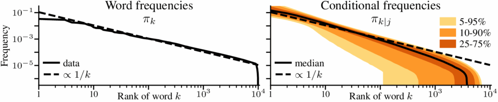
In the previous post [1], the eigenvalues and distances to the solution were assumed to follow power-laws. For this problem, this comes naturally if we assume that the marginal and conditional distributions of the tokens follow Zipf’s law. For the marginal distribution of the tokens \(x\), we assume that the tokens are sorted by frequency and that the \(i\)-th most frequent token has probability \(\pi_i \propto 1/i\). For the conditional distribution of the next token \(y\) following the \(i\)-th token, we assume the same Zipfian structure; if \(\rho_i(j)\) is the index of the \(j\)-th most frequent token after the \(i\)-th token, then \(\pi_{\rho_i(j) \,\vert\, i} \propto 1/j\). By \(\propto\) we mean that the probabilities are normalized to sum to 1, that is $$
\pi_i = \frac{1}{H_d} \frac{1}{i}
\quad \text{ and } \quad
\pi_{\rho_i(j)\,\vert\, i} = \frac{1}{H_d} \frac{1}{j}
\quad \text{ where } \quad
H_d = \sum_{i=1}^d \frac{1}{i}.
$$ This assumption simplifies the dynamics. As \(\pi_{\rho_i(j) \,\vert\, i}\) does not depend on \(i\), the \(d^2\)-dimensional problem can be written as a sum of \(d\) terms, $$
\begin{aligned}
F_d(W_k) \,-\, F_{d,*}
= \frac{1}{2} \sum_{i=1}^d \pi_i \left(1-\eta\pi_i\right)^{2k} \sum_{j=1}^d \pi_{j\,\vert\, i}^2
= \frac{1}{2H_d} \sum_{i=1}^d \frac{1}{i} \left(1-\frac{\eta}{H_d}\frac{1}{i}\right)^{2k} \frac{H_{d,2}}{H_d^2},
\end{aligned} $$ where \(H_{d,2} = \sum_{i=1}^d {1}/{i^2}\). The assumption on the marginal distribution \(\pi_i\) is just Zipf’s law, which describes language data even after tokenization [16, 17, 18]. The assumption on the conditional distribution is more of an approximation, but appears to be reasonable enough for our purposes, as shown below.

Getting a meaningful limit

We now look at what makes the analysis difficult. The first problem is that the optimality gap at initialization does not converge to a nice constant value as \(d \to \infty\). The second is that the difficulty of the problem increases as \(d\) increases, making it impossible to make progress as \(d \to \infty\). By fixing those problems, we will be able to show that $$
F_d(W_k) \,-\, F_{d,*} \approx \left(1-\frac{\log(2k)}{\log(d)}\right)\left(F_d(W_0) \,-\, F_{d,*}\right).
$$

Scaling at initialization

While for some models the optimality gap at initialization converges to a constant as \(d \to \infty\), for others the initial optimality gap depends heavily on the dimension \(d\). For the problem described above, the optimality gap at initialization is, using usual asymptotics of \(H_d \sim \log(d)\) and \(H_{d,2} \sim \pi^2/6\),
$$
F_d(W_k) \,-\, F_{d,*}
= \frac{1}{2} \frac{H_{d,2}}{H_d^2} \sim \frac{\pi^2}{12 \log(d)^2}.
$$ In this case, the optimality gap converges to zero because the eigenvalues are probabilities and are normalized to sum to 1. Without that normalization, the optimality gap at initialization would diverge instead, as is the case in the first figure. In either case, studying the optimality gap in the limit of \(d \to \infty\) is not meaningful.

But there is a way to normalize the problem to obtain a meaningful limit. Instead of looking at the optimality gap \(F_d(W_k) \,- F_{d,*}\), we can look at the normalized optimality gap $$
r_d(k) = \frac{F_d(W_k) \,-\, F_{d,*}}{F_d(W_0) \,-\, F_{d,*}}
\,\, \text{ such that } \,\,
F_d(W_k) \,-\, F_{d,*} = r_d(k) \cdot \left(F_d(W_0) \,-\, F_{d,*}\right), $$ The normalized optimality gap starts at \(r_d(0) = 1\) and goes to \(r_d(k) = 0\) as \(k \to \infty\) if gradient descent converges. It can be thought of as the percentage of the loss of the optimization problem that we still have to solve. The normalized optimality gap would be the same whether we normalize the eigenvalues to sum to 1 or not, reflecting the fact that the optimization dynamics are the same; the only difference is in the scale of the initial loss. Computing the normalized optimality gap \(r_d(k)\) “fixes” this scaling problem and gives a meaningful limit. For our problem, it is $$
\begin{aligned}
r_d(k)
= \frac{1}{H_d} \sum_{i=1}^d \frac{1}{i} \left(1-\frac{\eta}{H_d}\frac{1}{i}\right)^{2k}
= \frac{1}{H_d} \sum_{i=1}^d \frac{1}{i} \left(1-\frac{1}{i}\right)^{2k}
\quad \text{ if } \quad \eta = H_d,
\end{aligned}
$$ where we picked the step-size \(\eta = 1/h_1 = H_d\) where \(h_1\) is the largest eigenvalue. If we now plot the normalized optimality gap \(r_d(k)\) as a function of \(k\), the dynamics of gradient descent converge as \(d \to \infty\). The only remaining problem is that they converge to \(1\) (that is, no progress is made), regardless of the iteration counter \(k\). See below

Scaling time with dimension

The above plot suggest that the problem becomes more difficult as the dimension \(d\) increases. If we take \(d \to \infty\) while keeping \(k\) fixed, we have no chance of making progress. However, we might be able to make progress if we scale the number of iterations \(k\) with the dimension \(d\).

To make this formal, instead of working with the sum representation of the normalized optimality gap \(r_d(k)\), we introduce the integral approximation \(I_d(k)\) $$ I_d(k) = \frac{1}{H_d} \int_1^d \frac{1}{i} \left(1-\frac{1}{i}\right)^{2k} \mathrm{d}i
\qquad \approx \qquad
r_d(k) = \frac{1}{H_d} \sum_{i=1}^d \frac{1}{i} \left(1-\frac{1}{i}\right)^{2k}.
$$ To show that the discrete sum \(r_d(k)\) is asymptotically equivalent to the integral \(I_d(k)\) if \(d\) is large enough, we can use the fact that the integral of a monotone function is sandwiched by its left- and right-Riemannian sums. The integrand is not monotone, instead it is first monotone increasing then decreasing, but with a little bit of work we can use those properties to get $$ \left\vert r_d(k) \,-\, I_d(k)\right\vert \leq \max \left\{\frac{1}{ d \log(d)}, \frac{1}{ 2k \log(d)}\right\}.
$$ The error vanishes \(d \to \infty\), so \(r_d(k) \sim I_d(k)\) as long as the error \(r_d(k)\) remains finite. The integral is easier to read and manipulate than the sum, especially with the change of variable \(i = d^{z}\); $$
I_d(k)
= \frac{\log(d) }{H_d} \int_0^1 \left(1 \,-\, \frac{1}{d^z}\right)^{2k} \mathrm{d}z
\sim \int_0^1 \left(1 \,-\, \frac{1}{d^z}\right)^{2k} \mathrm{d}z.
$$ where we used the fact that \(H_d \sim \log(d)\). From this expression, we can see that we cannot make progress for a fixed \(k\) if \(d \to \infty\). Exchanging the limit and the integral (the dominated convergence theorem applies), $$
\lim_{d\to\infty} I_d(k)
= \int_0^1 \lim_{d\to\infty} \left(1 \,-\, \frac{1}{d^z}\right)^{2k} \mathrm{d}z
= \int_0^1 1 \, \mathrm{d}z = 1.
$$ However, we can make progress if the number of iterations \(k\) grows with \(d\). If we take \(k\) to grow linearly with \(d\), say \(2k = \tau d\) for some \(\tau > 0\) which acts as a “rescaled” time variable, then the limit becomes $$
\lim_{d\to\infty} I_d(k)
= \int_0^1 \lim_{d\to\infty} \left(1 \,-\, \frac{1}{d^z}\right)^{\tau d} \mathrm{d}z
= \int_0^1 \lim_{d\to\infty} \exp\left(-\tau d^{1-z}\right) \mathrm{d}z
= \int_0^1 0 \, \mathrm{d}z
= 0,
$$ i.e., we solve the problem completely. This indicates that \(k = \Theta(1)\) is too slow to make progress, while \(k = \Theta(d)\) is too fast and solves the problem immediately. The right scaling to obtain a non-degenerate limit is somewhere in between. We can get it by taking \(2k = d^{\tau}\) for some \(\tau \in [0,1]\), as $$
\lim_{d\to\infty} I_d(k)
= \int_0^1 \lim_{d\to\infty} \left(1 \,-\, \frac{1}{d^z}\right)^{d^{\tau}} \mathrm{d}z
= \int_0^1 \lim_{d\to\infty} \exp\left(-d^{\tau-z}\right) \mathrm{d}z
$$ The behavior of \(\exp\left(-d^r\right)\) as \(d \to \infty\) depends on \(r\). If \(r > 0\), \(d^r \to \infty\) and \(e^{-d^r} \to 0\) but if \(r < 0\), \(d^r \to 0\) and \(e^{-d^r} \to 1\). $$
\lim_{d\to\infty} I_d(k)
= \int_0^{\tau} 0 \, \mathrm{d}z + \int_{\tau}^1 1 \, \mathrm{d}z
= 1 – \tau.
$$ This gives us a meaningful limit that does not degenerate to 0 or 1. This result gives us that if we scale \(k\) as \(\frac{1}{2}d^\tau\) for \(\tau \in [0,1]\) we get the limit $$
r_d(k(\tau)) = \frac{F_d(W_{d^\tau}) \,-\, F_{d,*}}{F_d(W_0) \,-\, F_{d,*}} \sim 1 \, – \tau
\quad \text{ for } \quad
2k(\tau) = d^\tau.
$$ Using that \(\tau = \log(2k)/\log(d)\), for finite \(k\) and \(d\) we have approximately, as promised, $$
F_d(W_k) \,-\, F_{d,*} \approx \left(1-\frac{\log(2k)}{\log(d)}\right)\left(F_d(W_0) \,-\, F_{d,*}\right).
$$ Let’s cast this in terms of the amount of time required to reach a certain relative error. To get to a relative error of \(\epsilon\), we need \(1 – \tau = \epsilon\), or \(k = \frac{1}{2}d^{1-\epsilon}\) iterations. For a small relative \(\epsilon\), say \(\epsilon < 0.01\), the difficulty scales almost linearly with \(d\). This is in stark contrast with the problems studied in the previous post [1], where a scaling law of \(\Theta(1/k^p)\) meant that the time to reach a relative error of \(\epsilon\) was \(k = \Theta(1/\epsilon^{1/p})\), independent of \(d\). To verify that the scaling is correct, we plot below the normalized optimality gap \(r_d(k)\) as a function of the rescaled time \(\tau = \log(2k)/\log(d)\), and see that it indeed converges to the limit \(1-\tau\) as \(d\) grows. The following plot compares the dynamics in finite dimension when the eigenvalues follow our assumptions, and we check the results on real text data at the end of the post.

Summary. Typical scaling laws can break down when taking \(d\) to \(\infty\), either by diverging, converging to 0, or converging to a constant independent of the number of iterations \(k\). To get a meaningful description of the optimization dynamics, we can normalize and rescale the problem, and taking the number of iterations \(k\) to grow with \(d\) gives a well-defined limit.

Insights on next-token prediction problems

With the normalization presented above, we can answer new questions on the dynamics of optimization on high-dimensional problems.

Our motivation for this work [3] was to understand the optimization dynamics of different optimizers on next-token prediction problems. Multiple papers have shown experimentally that Adam outperforms SGD in the training of large language models, and that the margin was larger than on other problem classes like image classification [4, 5, 6, 7]. With this analysis, we can show that

• The problem with gradient descent comes from text data following Zipf’s law, which is “worst case” for the performance of gradient descent.
• Other algorithms, like sign descent, can outperform gradient descent by having a much better scaling with dimension.

Impact of the token distribution

Previous work had shown experimentally that the Zipfian distribution of tokens found in language data made optimization with gradient descent difficult [7]. With our scaling laws, we can show that Zipf’s law is indeed “worst case” for next-token prediction problems, in that across all power laws \(h_i \propto 1/i^\alpha\), the case \(\alpha = 1\) leads to the worst scaling between the number of iterations \(k\) and the vocabulary size.

In the presentation above, we assumed that the marginal and conditional distributions of the tokens followed Zipf’s law, i.e. \(\pi_i \propto 1/i\) and \(\pi_{\rho_i(j)\,\vert\, i} \propto 1/j\). To gain insights into how the distribution of the tokens affects the optimization dynamics, we can consider more general power laws, such as $$
\pi_i \propto \frac{1}{i^\alpha}
\quad \text{ and } \quad
\pi_{\rho_i(j)\,\vert\, i} \propto \frac{1}{j^\alpha}
\quad \text{ for } \quad
\alpha > 0.
$$ Zipf’s law corresponds to \(\alpha= 1\), which we have just done. The case \(\alpha > 1\) can be handled by the analysis in the previous post [1], and gives a sublinear rate independent of \(d\). The case \(\alpha < 1\) requires normalization, and using the same tools as above we can show that the required scaling is \(k = \Theta(d^\alpha)\) to get a non-degenerate limit (see the paper for more details [3]). This gives us the following table $$
\begin{aligned}
\begin{aligned}
\alpha &< 1
\\
k &= \Theta(d^\alpha)
\end{aligned}
&&
\begin{aligned}
\alpha &= 1
\\
k &= \Theta(d^{1-\epsilon})
\end{aligned}
&&
\begin{aligned}
\alpha &< 1
\\
k &= \Theta(1)
\end{aligned}
\end{aligned}
$$ The case \(\alpha \approx 1\) is “worst case” for next-token prediction problems in terms of the required number of iterations as a function of \(d\).

One intuition for the impact of \(\alpha\) is that if \(\alpha \gg 1\), the frequencies are very skewed and gradient descent is slow at learning the rare tokens, but the rare tokens contribute little to the overall loss and can be ignored. If \(\alpha \ll 1\), the frequencies are closer to uniform and gradient descent makes more progress on rare words. The case \(\alpha \approx 1\) is the hardest because the frequencies are skewed enough that gradient descent makes little progress on rare tokens and the rare tokens contribute significantly to the overall loss.

Dynamics of sign descent

High-dimensional analysis can also explain why Adam-like algorithms outperforms gradient descent on this problems. The update of the Adam algorithm is too complicated to give us closed-form solutions, but we can look at sign descent as a proxy. Previous work has shown that on problems where Adam outperforms gradient descent, sign descent also works well [6, 7], and the Adam update (simplified here to ignore bias correction) reduces to sign descent if we take some of its parameters to 0. It maintains two moving averages \(m_k\) and \(M_k\) of the gradient \(G_k\) and its (element-wise) square \(G_k^2\), and does the following update $$
\begin{aligned}
\begin{aligned}
m_{k+1} &= \beta_1 m_k + (1-\beta_1) G_k,
\\
M_{k+1} &= \beta_2 M_k + (1-\beta_2) G_k^2,
\end{aligned}
&&
W_{k+1} &= W_k \,-\, \eta \frac{m_{k+1}}{\sqrt{M_{k+1}} + \epsilon},
\end{aligned}
$$ where all the operations on vectors or matrices are element-wise. Ignoring the moving averages by taking \(\beta_1 = \beta_2 = 0\) and \(\epsilon = 0\), we get sign descent, $$
W_{k+1} = W_k \,-\, \eta \, \text{sign}(G_k).
$$ where \(\text{sign}(\cdot)\) is the element-wise sign function, giving \(+1\) or \(-1\) depending on the sign of the gradient.

Proving that sign descent outperforms gradient descent is typically difficult. The algorithm does not converge with a fixed step-size. It requires either a decreasing step-size or a small enough step-size that depends on the total number of steps taken. Most analyses under classical smooth/Lipschitz/convex assumptions give convergence rates that explicitly or implicitly have a poor dependence on the dimension \(d\) [20, 21, 22]. But using asymptotic analysis, we will be able to show that sign descent scales much better with the vocabulary size \(d\) than gradient descent, taking requiring the number of iterations to scale with \(\sqrt{d}\) instead of \(d\).

To do the analysis, we first need a closed-form solution for the dynamics of sign descent. Getting this closed-form is often out of reach because the update is non-linear, even on quadratics. But in this specific case, the Hessian is diagonal and there is no interaction between the different coordinates, which makes the analysis possible by looking at the effect of sign descent on each coordinate.

The broad strokes of the analysis are similar as the case for gradient descent. We first derive the dynamics of sign descent, with the added difficulty that we have to identify when the algorithm is converging monotonically versus when it is oscillating around the solution. For gradient descent, we could get close to optimal performance with a constant step-size by picking \(\eta = 1/h_1\). But sign descent with a fixed step-size ends up oscillating if run for long enough, so we need to scale the step-size \(\eta\) with \(d\) and \(k\) to get good performance. We leave the details to the paper, but we show that there is a step-size such that after \(K \propto \tau \sqrt{d}\) steps we reach an error of \(O(1/\tau^2)\). The dependence on the dimension is much better; \(\sqrt{d}\) instead of (almost) \(d\) for small \(\epsilon\), showing that sign descent with a properly chosen step-size can outperform gradient descent.

The analysis is of course limited, as the problem is quadratic and axis-aligned. But we have empirical evidence that the benefit of Adam in language transformers comes from its improvement over gradient descent in the first and last layers of the network [23, 24]. The problem is not too dissimilar from the diagonal quadratic problem we study as the imbalance in those layers comes from the token frequencies and is axis aligned along the axis of the weight matrix that corresponds to the vocabulary.

Conclusion

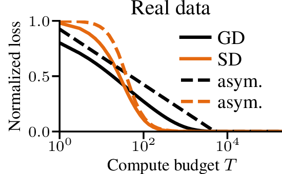
In this blog post, we discussed issues that arise in scaling law when the limit as \(d\) goes to \(\infty\) or converge trivially to 0, and how to normalize and rescale time to avoid those degenerate cases. We can use those tools to analyze settings that were not available before, like text data. Although we had to make some assumptions on the distributions, the behavior of gradient and sign descent on linear models with real text data is reasonably well approximated by the asymptotic prediction.

References

[1] Francis Bach. Scaling laws of optimization. Blog post, 2024.
[2] Francis Bach. Revisiting scaling laws via the z-transform. Blog post, 2025.
[3] Frederik Kunstner and Francis Bach. Scaling Laws for Gradient Descent and Sign Descent for Linear Bigram Models under Zipf’s Law. Preprint, arxiv:2505.19227, 2025.
[4] Jingzhao Zhang, Tianxing He, Suvrit Sra, and Ali Jadbabaie (2020a). Why Gradient Clipping Accelerates Training: A Theoretical Justification for Adaptivity. International Conference on Learning Representations (ICLR) 2020.
[5] Jingzhao Zhang, Sai Praneeth Karimireddy, Andreas Veit, Seungyeon Kim, Sashank J. Reddi, Sanjiv Kumar, and Suvrit Sra. Why are Adaptive Methods Good for Attention Models? Advances in Neural Information Processing Systems (NeurIPS) 2020.
[6] Frederik Kunstner, Jacques Chen, Jonathan Wilder Lavington, and Mark Schmidt. Noise is not the main factor behind the gap between SGD and Adam on transformers, but sign descent might be. International Conference on Learning Representations (ICLR) 2023.
[7] Frederik Kunstner, Alan Milligan, Robin Yadav, Mark Schmidt, and Alberto Bietti. Heavy-Tailed Class Imbalance and Why Adam Outperforms Gradient Descent on Language Models. Advances in Neural Information Processing Systems (NeurIPS) 2024.
[8] Andrea Caponnetto and Ernesto De Vito. Optimal Rates for the Regularized Least-Squares Algorithm. Foundations of Computational Mathematics 7.3, pp. 331–368.
[9] Raphaël Berthier, Francis R. Bach, and Pierre Gaillard. Tight Nonparametric Convergence Rates for Stochastic Gradient Descent under the Noiseless Linear Model. Advances in Neural Information Processing Systems (NeurIPS) 2020.
[10] Hugo Cui, Bruno Loureiro, Florent Krzakala, and Lenka Zdeborová. Generalization Error Rates in Kernel Regression: The Crossover from the Noiseless to Noisy Regime. Advances in Neural Information Processing Systems (NeurIPS) 2021.
[11] Alexander Maloney, Daniel A. Roberts, and James Sully. A Solvable Model of Neural Scaling Laws. Preprint arXiv/2210.16859 2022.
[12] Blake Bordelon, Alexander B. Atanasov, and Cengiz Pehlevan. A Dynamical Model of Neural Scaling Laws. International Conference on Machine Learning (ICML) 2024.
[13] Licong Lin, Jingfeng Wu, Sham M. Kakade, Peter L. Bartlett, and Jason D. Lee. Scaling Laws in Linear Regression: Compute, Parameters, and Data. Neural Information Processing Systems (NeurIPS) 2024.
[14] Elliot Paquette, Courtney Paquette, Lechao Xiao, and Jeffrey Pennington. 4+3 Phases of Compute-Optimal Neural Scaling Laws. Neural Information Processing Systems (NeurIPS) 2024.
[15] Yaroslav Bulatov. Gradient descent under harmonic eigenvalue decay. Blog post, 2023.
[16] Jonas F. Lotz, António V. Lopes, Stephan Peitz, Hendra Setiawan, Leonardo Emili. Beyond Text Compression: Evaluating Tokenizers Across Scales. Annual Meeting of the Association for Computational Linguistics (ACL) 2025.
[17] Yanjin He, Qingkai Zeng, Meng Jiang. Pre-trained Models Perform the Best When Token Distributions Follow Zipf’s Law. Annual Meeting of the Association for Computational Linguistics (ACL) 2025.
[18] Elizaveta Zhemchuzhina, Nikolai Filippov, Ivan P. Yamshchikov. Pragmatic Constraint on Distributional Semantics. Workshop on Knowledge Augmented Methods for NLP (KnowledgeNLP-AAAI 2023)
[19] Stefan Thurner, Rudolf Hanel, Bo Liu, and Bernat Corominas-Murtra. Understanding Zipf’s law of word frequencies through sample-space collapse in sentence formation. Journal of the Royal Society Interface, 2015.
[20] Jeremy Bernstein, Yu-Xiang Wang, Kamyar Azizzadenesheli, and Animashree Anandkumar. SIGNSGD: Compressed Optimisation for Non-Convex Problems. International Conference on Machine Learning (ICML) 2018.
[21] Yuxing Liu, Rui Pan, and Tong Zhang. AdaGrad under Anisotropic Smoothness. International Conference on Learning Representations (ICLR) 2025.
[22] Rudrajit Das, Naman Agarwal, Sujay Sanghavi, Inderjit S. Dhillon. Understanding the Preconditioning Effect of Adam in Deep Learning. Preprint, arxiv:2402.07114, 2024.
[23] Yushun Zhang, Congliang Chen, Ziniu Li, Tian Ding, Chenwei Wu, Diederik P. Kingma, Yinyu Ye, Zhi-Quan Luo, and Ruoyu Sun. Adam-mini: Use Fewer Learning Rates To Gain More. International Conference on Learning Representations (ICLR) 2025.
[24] Rosie Zhao, Depen Morwani, David Brandfonbrener, Nikhil Vyas, and Sham M. Kakade. Deconstructing What Makes a Good Optimizer for Autoregressive Language Models. International Conference on Learning Representations (ICLR) 2025.